DL 2 - Improving DNN: Hyperparameter tuning, Regularization and Optimization

Last modified on 01 Oct 2021.

This is my note for the course (Improving Deep Neural Networks: Hyperparameter tuning, Regularization and Optimization). The codes in this note are rewritten to be more clear and concise.

🎯 Overview of all 5 courses.

👉 Course 1 – Neural Networks and Deep Learning.
👉 Course 2 – Improving Deep Neural Networks: Hyperparameter tuning, Regularization and Optimization.
👉 Course 3 – Structuring Machine Learning Projects.
👉 Course 4 – Convolutional Neural Networks.
👉 Course 5 – Sequence Models.

This course will teach you the “magic” of getting deep learning to work well. Rather than the deep learning process being a black box, you will understand what drives performance, and be able to more systematically get good results. You will also learn TensorFlow.

Initialization step

layers_dims contains the size of each layer from $0$ to $L$.

zero initialization

parameters['W'+str(l)] = np.zeros((layers_dims[l], layers_dims[l-1]))
parameters['b'+str(l)] = np.zeros((layers_dims[l], 1))

• The performance is really bad, and the cost does not really decrease.
• initializing all the weights to zero ⇒ failing to break symmetry ⇒ every neuron in each layer will learn the same thing ⇒ $n^{[l]}=1$ for every layer ⇒ no more powerful than a linear classifier such as logistic regression.

Random initialization

To break symmetry, lets intialize the weights randomly.

parameters['W'+str(l)] = np.random.randn(layers_dims[l], layers_dims[l-1]) * 10 # <- LARGE (just an example of SHOULDN'T)
parameters['b'+str(l)] = np.zeros((layers_dims[l], 1))

• High initial weights ⇒ The cost starts very high (near 0 or 1 or infinity).
• Poor initialization ⇒ vanishing/exploding gradients ⇒ slows down the optimization algorithm.
• If you train this network longer ⇒ better results, BUT initializing with overly large random numbers ⇒ slows down the optimization.

He initialization

Multiply randomly initial $W$ with $\sqrt{\frac{2}{n^{[l-1]}}}$. It’s similar to Xavier initialization in which multipler factor is $\sqrt{\frac{1}{n^{[l-1]}}}$

parameters['W' + str(l)] = np.random.randn(layers_dims[l], layers_dims[l-1]) * np.sqrt(2./layers_dims[l-1])
parameters['b' + str(l)] = np.zeros((layers_dims[l], 1))

Regularization step

To reduce the overfitting problem.

L2 regularization

L2_regularization_cost = 0
for l in range(1, L+1):
    L2_regularization_cost += 1/m * lambd/2 * (np.sum(np.square(W[l]))

• The standard way. Modify cost function from, $J = -\frac{1}{m} \sum\limits_{i = 1}^{m} \large{(}\small y^{(i)}\log\left(a^{[L](i)}\right) + (1-y^{(i)})\log\left(1- a^{[L](i)}\right) \large{)}$ to $J_{regularized} = \small \underbrace{-\frac{1}{m} \sum\limits_{i = 1}^{m} \large{(}\small y^{(i)}\log\left(a^{[L](i)}\right) + (1-y^{(i)})\log\left(1- a^{[L](i)}\right) \large{)} }_\text{cross-entropy cost} + \underbrace{\frac{1}{m} \frac{\lambda}{2} \sum\limits_l\sum\limits_k\sum\limits_j W_{k,j}^{[l]2} }_\text{L2 regularization cost}$
• The value of $\lambda$ is a hyperparameter that you can tune using a dev set.
• L2 regularization makes your decision boundary smoother. If $\lambda$ is too large, it is also possible to “oversmooth”, resulting in a model with high bias.

Dropout

# [Forward] An example at layer 3
D3 = np.random.rand(A3.shape(0), A3.shape(1)) < keep_drop
A3 *= D3
A3 /= keep_drop
# [Backprop]
dA3 *= D3
dA3 /= keep_drop

• Dropout is a widely used regularization technique that is specific to deep learning.
• Randomly shuts down some neurons in each iteration.
• When you shut some neurons down, you actually modify your model. The idea behind drop-out is that at each iteration, you train a different model that uses only a subset of your neurons.
• With dropout, your neurons thus become less sensitive to the activation of one other specific neuron, because that other neuron might be shut down at any time.
• Don’t apply dropout to the input layer or output layer.
• Use dropout during training, not during test time.
• Apply dropout both during forward and backward propagation.

Gradient checking

• To answer “Give me a proof that your backpropagation is actually working!”
• We are confident on computing $J$ but $\frac{\partial J}{\partial\theta}$.
• Use $J$ to compute an approximation of $\frac{\partial J}{\partial\theta}$ and compare with $\frac{\partial J}{\partial\theta}$. $\frac{\partial J}{\partial \theta} = \lim_{\varepsilon \to 0} \frac{J(\theta + \varepsilon) - J(\theta - \varepsilon)}{2 \varepsilon}$

Optimization algorithms

Intuition:

• Gradient Descent: go down the hill.
• Momentum / RMSprop / Adam: which direction?

Mini-batch gradient descent

• Problem: NN works great on big data but many data leads to slow the training ⇒ We need to optimize!
• Solution: Divide into smaller “mini-batches” (for example, from 5M to 5K of 1K each).

$\begin{aligned} X_{(n_X, m=5M)} &= [\underbrace{X^{(1)},\ldots,X^{(1K)}}_{X^{\{1\}}_{(n_X,1K)}}, \underbrace{X^{(1K+1)},\ldots,X^{(2K)}}_{X^{\{2\}}_{(n_X,1K)}}, \ldots, \underbrace{X^{(m-1K+1)},\ldots,X^{(m)}}_{X^{\{5K\}}_{(n_X,1K)}}], \\ Y_{(1, m=5M)} &= [\underbrace{y^{(1)},\ldots,y^{(1K)}}_{Y^{\{1\}}_{(1,1K)}}, \underbrace{y^{(1K+1)},\ldots,y^{(2K)}}_{Y^{\{2\}}_{(1,1K)}}, \ldots, \underbrace{y^{(m-1K+1)},\ldots,y^{(m)}}_{Y^{\{5K\}}_{(1,1K)}}] \end{aligned}$

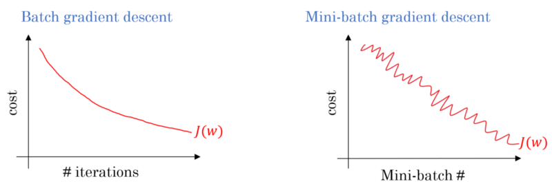Different between mini-batch and normal batch on the cost function. It’s oscillated for mini-batch because the cost may be large for this mini-batch but small for the others. Image from the course.

Notations

• $X^{(i)}$: $i$th training example.
• $z^{[l]}$: $z$ value in $l$th layer.
• $X^{\{t\}}, Y^{\{t\}}$: index of different mini-batches.

Algorithm

X = data_input
Y = labels
parameters = initialize_parameters(layers_dims)
for i in range(0, num_iterations): # loop through epoches: to get the convergence
    for t in range(0, num_batches): # loop through the batches
        # Forward propagation
        a, caches = forward_propagation(X[:,t], parameters)
        # Compute cost
        cost += compute_cost(a, Y[:,t])
        # Backward propagation
        grads = backward_propagation(a, caches, parameters)
        # Update parameters.
        parameters = update_parameters(parameters, grads)

How to build mini-batches?

We need 2 steps:

1. Shuffle: shuffle columns (training examples) correspondingly between $X$ and $Y$. The shuffling step ensures that examples will be split randomly into different mini-batches.
2. Partition: choose a batch size and take mini-batches. Note that, the last batch may be smaller than the others.

Type of mini-batch

There are 3 types based on the size of batches:

1. Batch Gradient Descent ($n_t = m$) : entire training examples, i.e. $(X^{\{1\}}, Y^{\{1\}}) = (X,Y)$.
2. Stochastic Gradient Descent ($n_t = 1$) : every training example is it own a mini-batch ($m$ mini batches).
3. $1<n_t<m$.

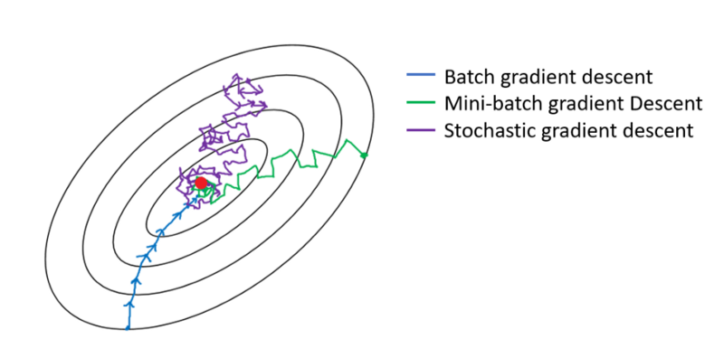Different between 3 types of mini-batch. Image from the course.

Guideline:

• If small training set ($m \le 2000$): using batch gradient descent.
• Typical mini-batch sizes: $64, 128, 256, 512, \ldots$
• Make sure mibi-batch size in CPU/GPU memory!

Exponentially weighted averages

• It’s faster than Gradient Descent!
• Example (temperature in London):
  • $\theta_t$: the temperature on day $t$.
  • $v_t$: the average temp of each day. It’s called exponential average over $\frac{1}{1-\beta}$ days temperature. $v_t = \beta v_{t-1} + (1-\beta)\theta_t$
  • E.g. $\beta=0.9 \Rightarrow v_t \simeq 10$ days temperature; $\beta=0.98 \Rightarrow v_t \simeq 50$ days temperature.
• $\beta$ larger ⇒ smoother average line because we consider more days. However, curve is now shifted further to the right.

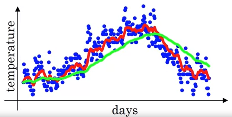Exponentially weighted average curves: red line ($\beta=0.9$), green line ($\beta=0.98$). Image from the course.

• When $\beta$ is so large ⇒ $v_t$ adapts slowly to the changes of temperature (more latency).
• Why we call “exponentially”? $\begin{aligned} v_{100} &= 0.9\times v_{99} + 0.1\times \theta_{100}\\ &= 0.1\times \theta_{100} + 0.1\times 0.99\times\theta_{99} + 0.1\times 0.99^2 \times\theta_{99} + \ldots \end{aligned}$

Bias correction

• Problem: the value of $v_t$ at the beginning of exp ave curves may be lower than what we expect. For example, with $v_0=0$, we have $v_1 = 0.02\theta_1$ instead of $v_1 = v_0 + 0.02\theta_1$.
• Solution: Instead of using $v_t$, we take $\dfrac{v_t}{1-\beta_t}$
• When $t$ is large ⇒ $\beta^t \simeq 0 \Rightarrow \dfrac{v_t}{1-\beta_t} \simeq v_t$

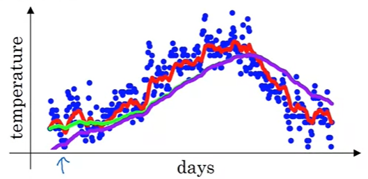Bias correction for the green line, it’s effective at the beginning of the line, with bigger $t$, green and violet are overlapped. Image from the course.

• In practice, we don’t really see people bothering with bias correction!

Gradient Descent with Momentum

• It’s faster than Gradient Descent!
• Why: when we use mini-batch, there are oscillation, momentum helps use reduce this.
• One sentence: compute the exponential weighted average of your gradient ⇒ use that gradient to update your weights instead.
• Idea: Momentum takes into account the past gradients to smooth out the update. We will store the ‘direction’ of the previous gradients in the variable $v$ . Formally, this will be the exponentially weighted average of the gradient on previous steps.
• Intuition: You can also think of $v$ as the “velocity” of a ball rolling downhill, building up speed (and momentum) according to the direction of the gradient/slope of the hill.
  • $dW, db$ like “acceleration”.
  • $VdW, Vdb$ like “velocity”.
  • $\beta$ likes “friction”.

We want slower learning in vertial direction and faster in horizontal direction. Image from the course.

• Algorithm: on iteration $t$:
  1. Compute $dW, db$ on current mini-batch.
  2. $VdW = \beta VdW + (1-\beta)dW$.
  3. $Vdb = \beta Vdb + (1-\beta)db$.
  4. $W:=W-\alpha VdW$.
  5. $b:=b-\alpha Vdb$.
• Implementation:
  • Try to tune between $[0.8; 0.999]$, commonly use $\beta=0.9$.
  • Don’t bother bias correction, NO NEED.
  • Don’t need $(1-\beta)$ in the formulas but Andrew prefer to keep it!
  • Bigger $\beta$, smaller in vertical direction.

RMSprop

• It’s “Root Mean Square propagation”.
• Algorithm: on iteration $t$,
  1. Compute $dW, db$ on current element-wise mini-batch.
  2. $SdW = \beta SdW + (1-\beta)dW^2$.
  3. $Sdb = \beta Sdb + (1-\beta)db^2$.
  4. $W:=W -\alpha \frac{dW}{\sqrt{SdW}+\epsilon}$.
  5. $b:=b-\alpha \frac{db}{\sqrt{SdW} + \epsilon}$.
• We choose $\epsilon=10^{-8}$ if $\sqrt{SdW}$ is too small, otherwise $\epsilon=0$.
• In practice: $dW, db$ are very high dimensional vectors.

Adam Optimization

• It’s “Adaptive Moment Estimation”.
• One of the most effective optimization algorithm for training NN. It’s commonly used and proven to be very effective for many different NN of a very wide variety of architectures.
• Adam = Momentum + RMSprop.
• Implementation: on iteration $t$,
  1. Compute $dW, db$ using current mini-batch.
  2. (Monentum) $VdW = \beta_1 VdW + (1-\beta_1)dW$; $Vdb = \beta_1 Vdb+(1-\beta_1)db$.
  3. (RMSprop) $SdW = \beta_2 SdW + (1-\beta_2)dW^2$; $Sdb = \beta_2Sdb +(1-\beta_2)db^2$.
  4. $V_{dW}^{\text{corrected}} = \dfrac{VdW}{1-\beta_1^t}$; $V_{db}^{\text{corrected}} = \dfrac{Vdb}{1-\beta_1^t}$.
  5. $S_{dW}^{\text{corrected}} = \dfrac{SdW}{1-\beta_2^t}$; $S_{db}^{\text{corrected}} = \dfrac{Sdb}{1-\beta_2^t}$.
  6. $W:=W-\alpha \dfrac{V_{dW}^{\text{corrected}}}{\sqrt{S_{dW}^{\text{corrected}}} + \epsilon}$; $b:=b-\alpha \dfrac{V_{db}^{\text{corrected}}}{\sqrt{S_{db}^{\text{corrected}}} + \epsilon}$.
• Initialization of the velocity is zero, i.e. $VdW=SdW=Vdb=Sdb=0$.
• If $\beta=0$, it’s standard gradient descent without momentum.
• Hyperparameter choices:
  • $\alpha$ = needs to be tuned, very important!
  • $\beta_1 = 0.9$ ($dW$), first moment.
  • $\beta_2 = 0.999$ ($dW^2$), second mement.
  • $\epsilon = 10^{-8}$.

Learning rate decay

• Idea: slowly reduce learning rate over time, it’s learning rate decay.
• Why? Below figure showes that, we need slower rate $\alpha$ (smaller step) at the area near the center.

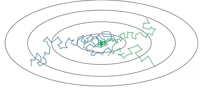Example of learning rate decay. Image from the course.

• Recall that, 1 epoch = 1 pass through data.
• Learning rate decay can be chosen 1 of below,

$\begin{aligned} \alpha &= \dfrac{1}{1 + \text{decay\_rate} \times \text{epoch\_num}} \times \alpha_0, \\ \alpha &= 0.95^{\text{epoch\_num}} \times \alpha_0 - \text{exponentially\_decay}, \\ \alpha &= \dfrac{k}{\sqrt{\text{epoch\_number}}} \times \alpha, \\ \alpha &= \dfrac{k}{\sqrt{t}} \times \alpha_0. \end{aligned}$

Problem of local optima

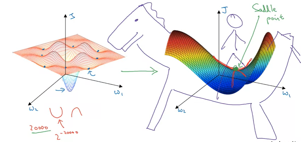Local optima problem: local & right optima (left) and saddle point (right). Image from the course.

• In high dimension, you likely see saddle points than local optimum.
• Problem of plateau: a region where derivative is close to zero for a long time.
  • Unlikely get stuck in a bad local optimal.
  • Plateau can make learning slow: use Momentum, RMSprop, Adam.

Batch GD makes learning too long?

• Try better random initialization for weights.
• Try mini-batch GD.
• Try using Adam
• Try tuning learning rate $\alpha$.

Hyperparameter tuning

Tuning process

• There are many hyperparameters but some are more important than others!
• Learning rate $\alpha$ (most important), #hiddien units, $\beta$, mini-batch size (2nd important), #layers, learning decay,…
• Don’t use grid, use random!

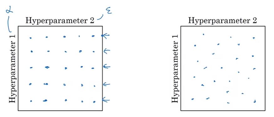Tuning process. Don’t use grid (left), use random (right). Image from the course.

• Coarse to fine: find an area containing effective values ⇒ zoom in and take more points in that area,

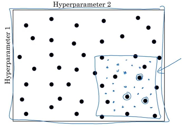Coarse to fine: first try on a big square, then focus on the smaller one (blue). Image from the course.

• Choose randomly but NOT mean uniform scale! We can choose uniformly on #hidden units, #layers, but not for the others (e.g. $\alpha$).
• For $\alpha$, for example, we need to divide into equal “large” spaces and then use uniform.

Appropriate scale for hyperparameters. Image from the course.

• Hyperparameters for exponentially weighted averages:
  • We cannot try with values between $[0.9, 0.999]$ because,
    • $\beta: 0.9000 \to 0.9005$ : no much changes,
    • $\beta: 0.999 \to 0.995$ : huge impact!

  • Consider $1-\beta \in [10^{-1}, 10^{-3}]$ instead!

    $\begin{aligned} r &\in [-3, -1] \\ 1-\beta = 10^r &\Leftrightarrow \beta = 1-10^r \end{aligned}$

In practice: Panda vs Caviar

• How to organize your hyperparameter search?
• Advice: Re-testing/Re-evaluating your hyperparameters at least once every several months.
• 2 ways:
  1. Babysitting one model (Panda): when we have huge data but weak CPU/GPU $\Rightarrow$ try very small number of models at a time. Check the performance step by step (cost function reduces…)
     • In some domains like advertising, computer vision apps,…
     • We call “panda” because panda has very few number of babies at a time (and in their life) $\Rightarrow$ try to keep them alike once at a time.
  2. Training many models in parallel (Caviar): when we don’t work on huge data + strong CPU/GPU. $\Rightarrow$ Try many models in parallel and choose the best performance!
     • We call “Caviar” because of intuition.

Batch Normalization

• Make NN much more robust to the choice of hyperparameters. $\Leftarrow$ doesn’t work for all NN but if it does, make training faster!
• One of the most important ideas in the rise of Deep Learning.
• Like we wanna normalize input to speed up learning, in this case, we wanna normalize $Z$ (in the hidden layers)

• If we choose different $\beta, \gamma$ $\Rightarrow$ hidden units have other means & variances.
• Instead of using $Z^{[l](1)}, \ldots, Z^{[l](m)}$, we use $\tilde{Z}^{[l](i)}$.
• Difference between normalizing input $X$ and normalizing in hidden units:
  • $X$: after normalizing, $\mu=0, \sigma=1$.
  • $Z$: after normalizing, various $\mu, \sigma$.

$X \xrightarrow[]{W^{[1]}, b^{[1]}} Z^{[1]} \xrightarrow[\text{Batch Norm}]{\beta^{[1]}, \gamma^{[1]}} \tilde{Z}^{[1]} \to a^{[1]} = g^{[1]}(\tilde{Z}^{[1]}) \xrightarrow[]{W^{[2]}, b^{[2]}} Z^{[2]} \xrightarrow[\text{Batch Norm}]{\beta^{[2]}, \gamma^{[2]}} \tilde{Z}^{[2]} \to a^{[2]} \to \ldots$

• Note that, $\beta$ in this case is different from $\beta$ in Adam optimization!
• We can use gradient descent to update $\beta$ and even use Adam/RMSprop/Momentum to update params $\gamma, \beta$, not just for Gradient Descent.
• In practice, we won’t have to implement Batch Norm step by step by ourself, programming framework (like Tensorflow) will do!
• In practice, Batch Norm is usually applied with mini-batch of your training set.
• Parameters: $W^{[l]}, \beta^{[l]}, \gamma^{[l]}$. We don’t need to consider $b^{[l]}$ becase it will be subtracted out in the process of normalization!
• Fitting Batch Norm into a NN: for $t$ goes through the number of mini-batches,
  1. Compute forward prop on $X^{\{t\}}$.
  2. In each hidden layer, use Batch Norm to reparameter $Z^{[l]}$ to $\tilde{Z}^{[l]}$.
  3. Use backprop to compute $dW^{[l]}, d\beta^{[l]}, d\gamma^{[l]}$.

  4. Update params (we can use Momentum / RMSprop / Adam):

     $\begin{aligned} W^{[l]} &:= W^{[l]} - \alpha dW^{[l]}, \\ \beta^{[l]} &:= \beta^{[l]} - \alpha d\beta^{[l]}, \\ \gamma^{[l]} &:= \gamma^{[l]} - \alpha d\gamma^{[l]}. \end{aligned}$

• Sometimes, BN has a 2nd effect as a regularization technique but it’s unintended! We don’t use it for the purpose of regularization, use L1, L2 or dropout instead.

Why BN works?

• Make weights in later / deeper layers be more robust to changing to the weights in the earlier layers.
• Covariate shift problem: suppose we have $X \to Y$. If $X$’s distribution changes, it changes the result in $Y$ much. We have to re-train our model.
  • Example: “cat vs non-cat” problem. If we apply params from the model of “black cat vs non-cat” to the problem of “colored-cat vs non-cat”, it won’t work because distribution in “black cat” is different from “colored cat”.

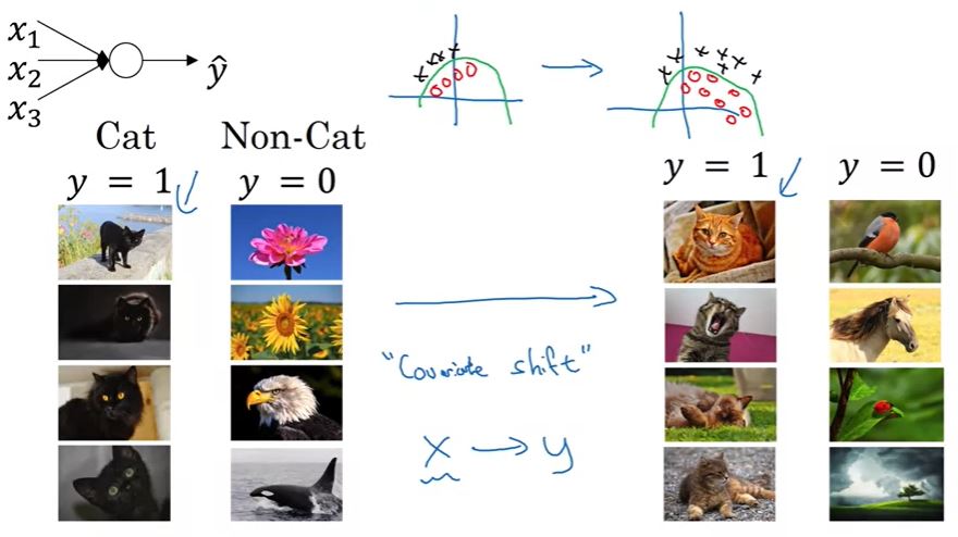Covariate problem. Image from the course.

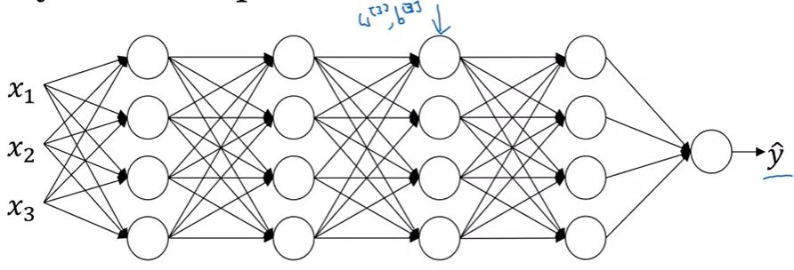Why BN works?. Image from the course.

In the perspective of layer 3, it depends only on layer 2 $\Rightarrow$ If layers before layer 2 changes $\Rightarrow$ distribution of layer 2 changes $\Rightarrow$ covariate shift problem for layer 3 $\Rightarrow$ Batch Norm makes sure that mean and variance in layer 2 is always robust before going to layer 3!

Batch Norm in test time

• BN processes our data one min-batch at a time. However, in test time, you need to process the examples at a time. $\Rightarrow$ Need to adapt your network to do that.
• Idea: calculate $\mu, \sigma^2$ using exponentially weighted average (across mini-batches). Other words,
  • In the training time, we calculate (and store) also the $\mu^{\{t\}[l]}, \sigma^{\{t\}[l]}$ in each mini-batch.
  • Find $\mu, \sigma^2$ (exponentially weighted average) of all mini-batches.
  • Use this $\mu, \sigma^2$ to find $Z_{\text{norm}}$ and $\tilde{Z}$ (at each example $i$).
• Don't worry, it's easy to use with Deep Learning Frameworks.

Tensorflow introduction

Writing and running programs in TensorFlow has the following steps:

1. Create Tensors (variables) that are not yet executed/evaluated.
2. Write operations between those Tensors.
3. Initialize your Tensors.
4. Create a Session.
5. Run the Session. This will run the operations you’d written above.

# create placeholders
x = tf.placeholder(tf.int64, name = 'x')
X = tf.placeholder(tf.float32, [n_x, None], name="X")

# initialize
W1 = tf.get_variable("W1", [25,12288], initializer = tf.contrib.layers.xavier_initializer(seed = 1))
b1 = tf.get_variable("b1", [25,1], initializer = tf.zeros_initializer())

There are two typical ways to create and use sessions in tensorflow:

1. Method 1:

    sess = tf.Session()
    # Run the variables initialization (if needed), run the operations
    result = sess.run(..., feed_dict = {...})
    sess.close() # Close the session
   

2. Method 2:

    with tf.Session() as sess:
        # run the variables initialization (if needed), run the operations
        result = sess.run(..., feed_dict = {...})
        # This takes care of closing the session for you :)
   

What you should remember:

• Tensorflow is a programming framework used in deep learning
• The two main object classes in tensorflow are Tensors and Operators.
• When you code in tensorflow you have to take the following steps:
  • Create a graph containing Tensors (Variables, Placeholders …) and Operations (tf.matmul, tf.add, …)
  • Create a session
  • Initialize the session
  • Run the session to execute the graph
• You can execute the graph multiple times as you’ve seen in model()
• The backpropagation and optimization is automatically done when running the session on the “optimizer” object.

👉 Check more details about the codes in the notebook.

👉 Course 3 – Structuring Machine Learning Projects.

×Close