Thi | DL 1 - NN and DL

Last modified on 01 Oct 2021.

This is my note for the course (Neural Networks and Deep Learning). The codes in this note are rewritten to be more clear and concise.

🎯 Overview of all 5 courses.

👉 Course 1 – Neural Networks and Deep Learning.
👉 Course 2 – Improving Deep Neural Networks: Hyperparameter tuning, Regularization and Optimization.
👉 Course 3 – Structuring Machine Learning Projects.
👉 Course 4 – Convolutional Neural Networks.
👉 Course 5 – Sequence Models.

If you want to break into cutting-edge AI, this course will help you do so.

Activation functions

Check Comparison of activation functions on wikipedia.

Why non-linear activation functions in NN Model?

Suppose $g(z)=z$ (linear)

$\begin{aligned} a^{[1]} &= g(z^{[1]} = z^{[1]}) = w^{[1]}x + b^{[1]} \quad \text{(linear)} \\ a^{[1]} &= g(z^{[2]} = z^{[2]}) = w^{[2]}a^{[1]} + b^{[2]} \\ &= (w^{[2]}w^{[1]})x + (w^{[2]}b^{[1]} + b^{[2]}) \quad \text{(linear again)}. \end{aligned}$

You might not have any hidden layer! Your model is just Logistic Regression, no hidden unit! Just use non-linear activations for hidden layers!

Sigmoid function

Usually used in the output layer in the binary classification.
Don't use sigmoid in the hidden layers!

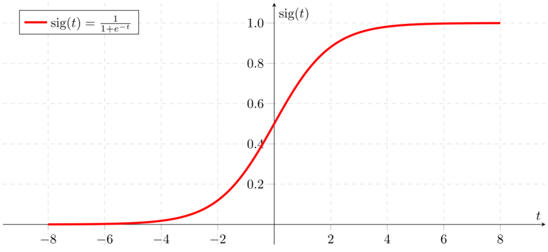$\begin{aligned} \sigma(z) &= \dfrac{1}{1+e^{-z}} \\ \sigma(z) &\xrightarrow{z\to \infty} 1 \\ \sigma(z) &\xrightarrow{z\to -\infty} 0 \\ \sigma'(x) &= \sigma(x) (1 - \sigma(x)) \end{aligned}$

sigmoid function Signmoid function graph on Wikipedia.

import numpy as np
import numpy as np

def sigmoid(z):
    return 1 / (1+np.exp(-z))

def sigmoid_derivative(z):
    return sigmoid(z)*(1-sigmoid(z))

Softmax function

The output of the softmax function can be used to represent a categorical distribution – that is, a probability distribution over K different possible outcomes.

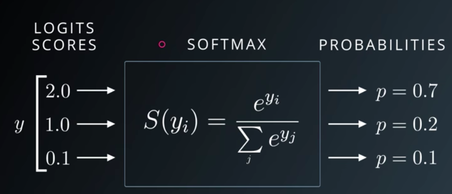softmax function Udacity Deep Learning Slide on Softmax

$\sigma (\mathbf {z} )_{i}={\frac {e^{z_{i}}}{\sum _{j=1}^{K}e^{z_{j}}}}{\text{ for }}i=1,\dotsc ,K{\text{ and }}\mathbf {z}\in \mathbb {R} ^{K}$

def softmax(x):
    z_exp = np.exp(z)
    z_sum = np.sum(z_exp, axis=1, keepdims=True)
    return z_exp / z_sum

tanh function (Hyperbolic tangent)

tanh is better than sigmoid because mean $\to$ 0 and it centers the data better for the next layer.
Don’t use sigmoid on hidden units except for the output layer because in the case $0 \le \hat{y} \le 1$ , sigmoid is better than tanh.

$\sigma(z) = \dfrac{e^{z} - e^{-z}}{e^{z} + e^{-z}}$

def tanh(z):
    return (np.exp(z) - np.exp(-z)) / (np.exp(z) + np.exp(-z))

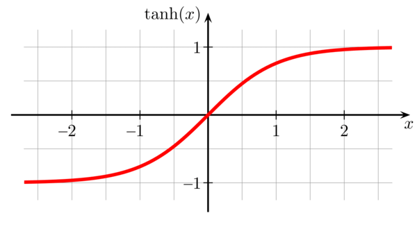tanh function Graph of tanh from analyticsindiamag.

ReLU

ReLU (Rectified Linear Unit).
Its derivative is much different from 0 than sigmoid/tanh $\to$ learn faster!
If you aren't sure which one to use in the activation, use ReLU!
Weakness: derivative ~ 0 in the negative side, we use Leaky ReLU instead! However, Leaky ReLU aren’t used much in practice!

$\sigma(z) = max(0,z)$

def relu(z):
    return np.maximum(0, z)

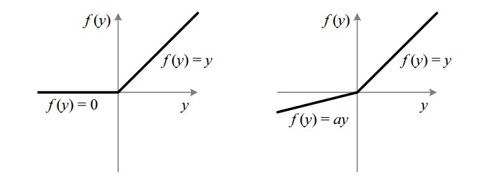relu vs leaky relu ReLU (left) and Leaky ReLU (right)

Logistic Regression

Usually used for binary classification (there are only 2 only 2 outputs). In the case of multiclass classification, we can use one vs all (couple multiple logistic regression steps).

Gradient Descent

Gradient Descent is an algorithm to minimizing the cose function $J$ . It contains 2 steps: Forward Propagation (From $X$ to compute the cost $J$ ) and Backward Propagation (compute derivaties and optimize the parameters $w, b$ ).

Initialize $w, b$ and then repeat until convergence ( $m$ : number of training examples, $\alpha$ : learning rate, $J$ : cost function, $A$ : activation function):

$A = \sigma(w^TX + b)$
$J(w,b) = -\frac{1}{m} \left( Y \log A^T + (1-Y)\log(1-A^T) \right)$
$\partial_{w}J = \frac{1}{m}X(A-Y)^T$
$\partial_{b}J = \frac{1}{m} \Sigma (A-Y)$
$w := w - \alpha \partial_{w}J$
$b := b - \alpha \partial_{b}J$

The dimension of variables: $X\in \mathbb{R}^{n_x \times m}, Y\in \mathbb{R}^{1\times m}, b\in \mathbb{R}^{1\times m}, w\in \mathbb{R}^{n_x \times 1}, A\in \mathbb{R}^{1\times m}, J\in \mathbb{R}$ , $\partial_wJ \in \mathbb{R}$ , $\partial_bJ \in \mathbb{R}$ .

Code

def logistic_regression_model(X_train, Y_train, X_test, Y_test,
                              num_iterations = 2000, learning_rate = 0.5):
    m = X_train.shape[1] # number of training examples

    # INITIALIZE w, b
    w = np.zeros((X_train.shape[0], 1))
    b = 0

    # GRADIENT DESCENT
    for i in range(num_iterations):
        # FORWARD PROPAGATION (from x to cost)
        A = sigmoid(np.dot(w.T, X_train) + b)
        cost = -1/m * (np.dot(Y, np.log(A.T))
               + p.dot((1-Y), np.log(1-A.T)))

        # BACKWARD PROPAGATION (find grad)
        dw = 1/m * np.dot(X_train, (A-Y).T)
        db = 1/m * np.sum(A-Y)
        cost = np.squeeze(cost)

        # OPTIMIZE
        w = w - learning_rate*dw
        b = b - learning_rate*db

    # PREDICT (with optimized w, b)
    Y_pred = np.zeros((1,m))
    w = w.reshape(X.shape[0], 1)

    A = sigmoid(np.dot(w.T,X_test) + b)
    Y_pred_test = A > 0.5

Neural Network overview

Notations

$X^{(i)}$ : $i$ th training example.
$m$ : number of examples.
$L$ : number of layers.
$n^{[0]} = n_X$ : number of features (# nodes in the input).
$n^{[L]}$ : number of nodes in the output layer.
$n^{[l]}$ : number of nodes in the hidden layers.
$w^{[l]}$ : weights for $z^{[l]}$ .
$a^{[0]} = X$ : activation in the input layer.
$a^{[2]}_i$ : activation in layer $2$ , node $i$ .
$a^{[2](i)}$ : activation in layer $2$ , example $i$ .
$a^{[L]} = \hat{y}$ .

Dimensions

$A^{[0]} = X \in \mathbb{R}^{n^{[0]} \times m}$
$Z^{[l]}, A^{[l]} \in \mathbb{R}^{n^{[l]}\times m}$ .
$dZ^{[l]}, dA^{[l]} \in \mathbb{R}^{n^{[l]}\times m}$ .
$dW^{[l]}, W^{[l]} \in \mathbb{R}^{n^{[l]} \times ^{[l-1]}}$ .
$db^{[l]}, b^{[l]} \in \mathbb{R}^{n^{[l]} \times 1}$ .

L-layer deep neural network

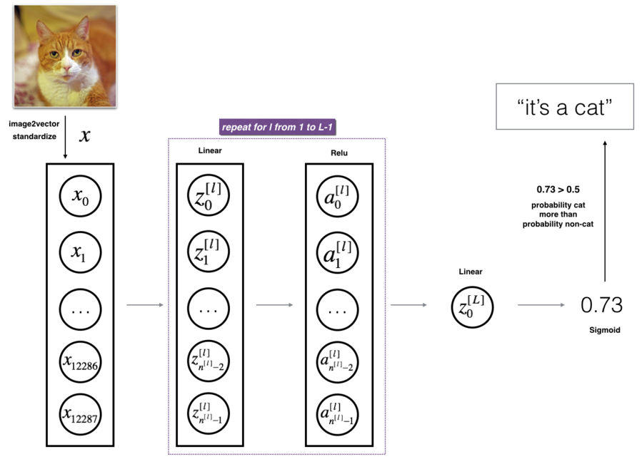L-layer deep neural network. Image from the course.

Initialize parameters / Define hyperparameters
Loop for num_iterations:
1. Forward propagation
2. Compute cost function
3. Backward propagation
4. Update parameters (using parameters, and grads from backprop)
Use trained parameters to predict labels.

Initialize parameters

In the Logistic Regression, we use $0$ for $w, b$ (it’s OK because LR doesn’t have hidden layers) but we can’t in the NN model!
If we use $0$ , we’ll meet the completely symmetric problem. No matter how long you train your NN, hidden units compute exactly the same function $\Rightarrow$ No point to having more than 1 hidden unit!
We add a little bit in $W$ and keep $0$ in $b$ .

Forward & Backward Propagation

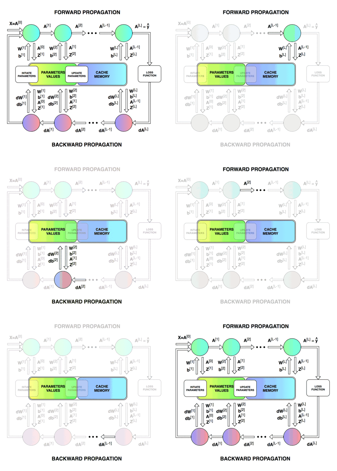Blocks of forward and backward propagation deep NN. Unknown source.

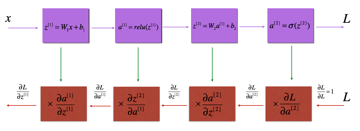Blocks of forward and backward propagation deep NN. Image from the course.

Forward Propagation: Loop through number of layers

$A^{[0]} = X$
$Z^{[l]} = W^{[l]}A^{[l-1]} + b^{[l]}$ (linear)
$A^{[l]} = \sigma^{[l]}(Z^{[l]})$ (for $l=1 \ldots L-1$ , non-linear activations)
$A^{[L]} = \sigma^{[L]}(Z^{[L]})$ (sigmoid function)

Cost function: $J(w,b) = -\frac{1}{m} \left( Y \log A^T + (1-Y)\log(1-A^T) \right)$

Backward Propagation: Loop through number of layers

$dA^{[L]} = -\frac{y}{A^{[L]}} + \frac{1-y}{1-A^{[L]}}$ .
for $l=L \ldots 1$ $l = L \dots 1$ , non-linear activations:
1. $dZ^{[l]} = dA^{[l]} (\sigma^{[l]})'(Z^{[l]})$ .
2. $dW^{[l]} = \frac{dJ}{\partial W^{[l]}} = \frac{1}{m} dZ^{[l]} (A^{[l-1])^T}$ .
3. $db^{[l]} = \frac{dJ}{\partial b^{[l]}} = \frac{1}{m}\sigma_1^m dZ^{[l](i)}$ .
4. $dA^{[l-1]} = (W^{[l])^T}dZ^{[l]}$ .

Update parameters: loop through number of layers (for $l=1\ldots L$ )

$W^{[l]} = W^{[l]} - \alpha dW^{[l]}$ .
$b^{[l]} = b^{[l]} - \alpha db^{[l]}$ .

Code

def L_Layer_NN(X, Y, layers_dims, learning_rate=0.0075,
               num_iterations=3000, print_cost=False):
    costs = []
    m = X_train.shape[1] # number of training examples
    L = len(layer_dims)  # number of layers

    # INITIALIZE W, b
    params = {'W':[], 'b':[]}
    for l in range(L):
        params['W'][l] = np.random.randn(layer_dims[l], layer_dims[l-1]) * 0.01
        params['b'][l] = np.zeros((layer_dims[l], 1))

    # GRADIENT DESCENT
    for i in range(0, num_iterations):
        # FORWARD PROPAGATION (Linear -> ReLU x (L-1) -> Linear -> Sigmoid (L))
        A = X
        caches = {'A':[], 'W':[], 'b':[], 'Z':[]}
        for l in range(L):
            caches['A_prev'].append(A)
            # INITIALIZE W, b
            W = params['W'][l]
            b = params['b'][l]
            caches['W'].append(W)
            caches['b'].append(b)
            # RELU X (L-1)
            Z = np.dot(W, A) + b
            if l != L: # hidden layers
                A = relu(Z)
            else: # output layer
                A = sigmoid(Z)
            caches['Z'].append(Z)

        # COST
        cost = -1/m * np.dot(np.log(A), Y.T) - 1/m * np.dot(np.log(1-A), 1-Y.T)

        #FORWARD PROPAGATION (Linear -> ReLU x (L-1) -> Linear -> Sigmoid (L))
        dA = - (np.divide(Y, A) - np.divide(1 - Y, 1 - A))
        grads = {'dW':[], 'db':[]}
        for l in reversed(range(L)):
            cache_Z = caches['Z'][l]
            if l != L-1: # hidden layers
                dZ = np.array(dA, copy=True)
                dZ[Z <= 0] = 0
            else: # output layer
                dZ = dA * sigmoid(cache_Z)*(1-sigmoid(cache_Z))
            cache_A_prev = caches['A_prev'][l]
            dW = 1/m * np.dot(dZ, cache_A_prev.T)
            db = 1/m * np.sum(dZ, axis=1, keepdims=True)
            dA = np.dot(W.T, dZ)
            grads['dW'].append(dW)
            grads['db'].append(db)

        # UPDATE PARAMETERS
        for l in range(L):
            params['W'][l+1] = params['W'][l] - grads['dW'][l]
            params['b'][l+1] = params['b'][l] - grads['db'][l]

    if print_cost and i % 100 == 0:
        print ("Cost after iteration %i: %f" %(i, cost))
    if print_cost and i % 100 == 0:
        costs.append(cost)

    return parameter

Parameters vs Hyperparameters

Parameters: $W, b$ .
Hyperparameters:
- Learning rate ( $\alpha$ ).
- Number of iterations (in gradient descent algorithm) ( $num_iterations$ ).
- Number of layers ( $L$ ).
- Number of nodes in each layer ( $n^{[i]}$ ).
- Choice of activation functions (their form, not their values).

Comments

Always use vectorized if possible! Especially for number of examples!
We can’t use vectorized for number of layers, we need for.
Sometimes, functions computed with Deep NN (more layers, fewer nodes in each layer) is better than Shallow (fewer layers, more nodes). E.g. function XOR.
Deeper layer in the network, more complex features to be determined!
Applied deep learning is a very empirical process! Best values depend much on data, algorithms, hyperparameters, CPU, GPU,…
Learning algorithm works sometimes from data, not from your thousands line of codes (surprise!!!)

Application: recognize a cat

This section contains an idea, not a complete task!

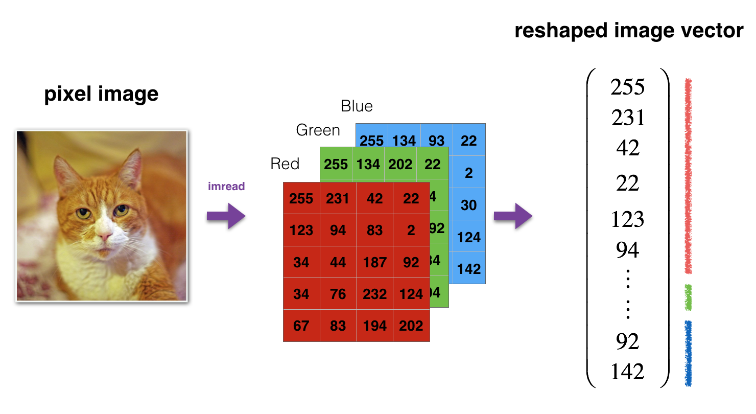Image to vector conversion. Image from the course.

L-layer deep neural network. Image from the course.

Python tips

○ Reshape quickly from (10,9,9,3) to (9*9*3,10):

X = np.random.rand(10, 9, 9, 3)
X = X.reshape(10,-1).T

○ Don’t use loop, use vectorization!

👉 Course 2 – Improving Deep Neural Networks: Hyperparameter tuning, Regularization and Optimization.