Last modified on 01 Oct 2021.
This is my note for the 4th course of TensorFlow in Practice Specialization given by deeplearning.ai and taught by Laurence Moroney on Coursera.
👉 Check the codes on my Github.
👉 Official notebooks on Github.
👉 Go to course 1 - Intro to TensorFlow for AI, ML, DL.
👉 Go to course 2 - CNN in TensorFlow.
👉 Go to course 3 - NLP in Tensorflow.
- Sequence models: focus on time series (there are others) – stock, weather,…
- At the end, we wanna model sunspot actitivity cycles which is important to NASA and other space agencies.
- Using RNN on time series data.
Sequences and prediction
Time Series
👉 Notebook: introduction to time series. + explaining video. => How to create synthetic time series data + plot them.
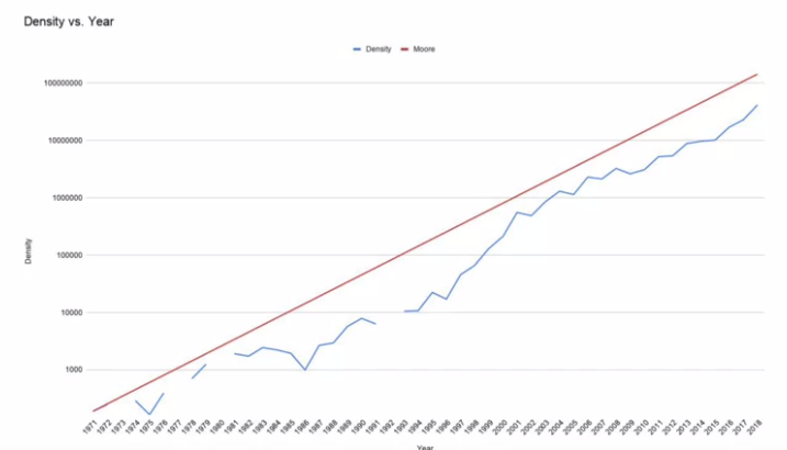
- Time series is everywhere: stock prices, weather focasts, historical trends (Moore’s law),…
- Univariate TS and Miltivariate TS.
- Type of things can we do with ML over TS:
- Any thing has a time factor can be analysed using TS.
- Predicting a focasting (eg. birth & death in Japan -> predict future for retirement, immigration, impacts…).
- Imputation: project back into the past.
- Fill holes in the data.
- Nomalies detecction (website attacks).
- Spot patterns (eg. speed recognition).
- Common patterns in TS:
-
Trend: a specific direcion that they’re moving in.
-
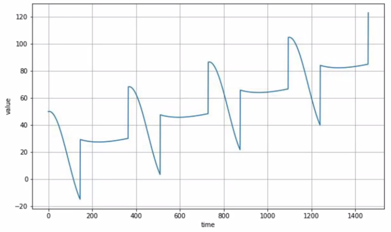
Seasonality: patterns repeat at predictable intervals (eg. active users for a website).

-
Combinition of both trend and seasonality.
-
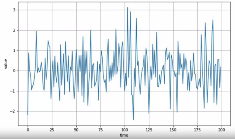
Stationary TS.
-
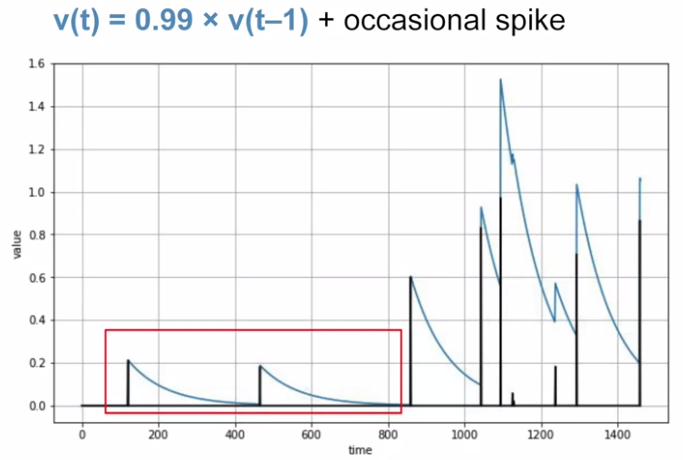
Autocorrelated TS: a time series is linearly related to a lagged version of itself.. There is no trend, no seasonality.
-
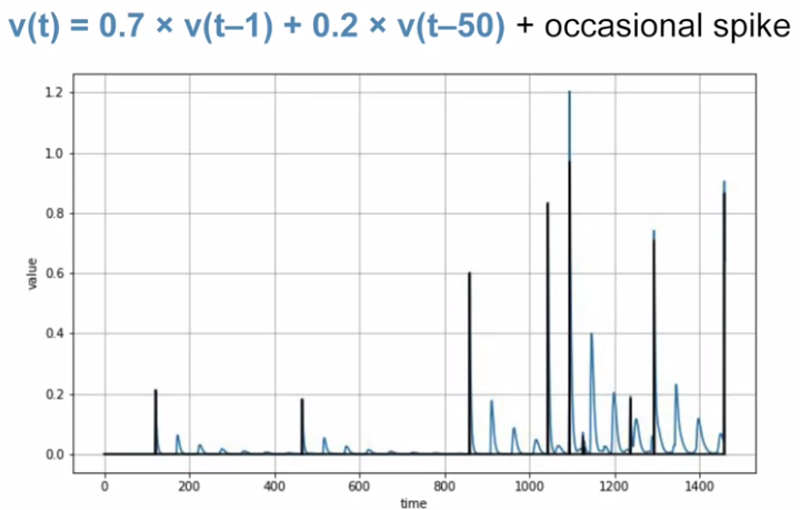
Multiple auto correlation.
-
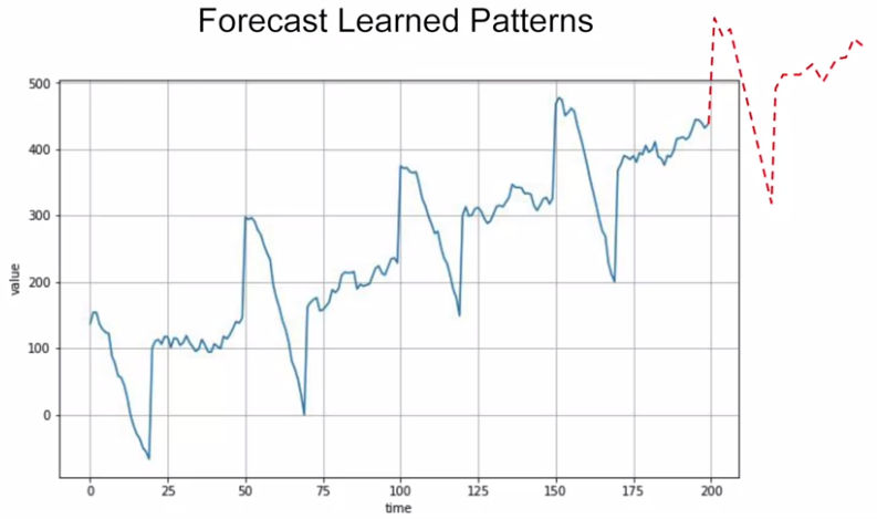
May be trend + seasonality + autorrelation + noise.
-
Non-stationary TS:
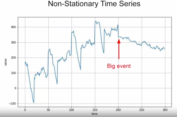 In this case, we base just on the later data to predict the future (not on the whole data).
-
Train / Validation / Test
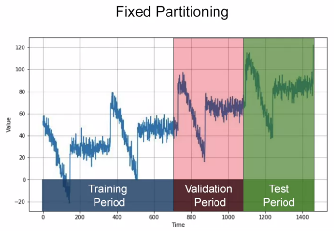
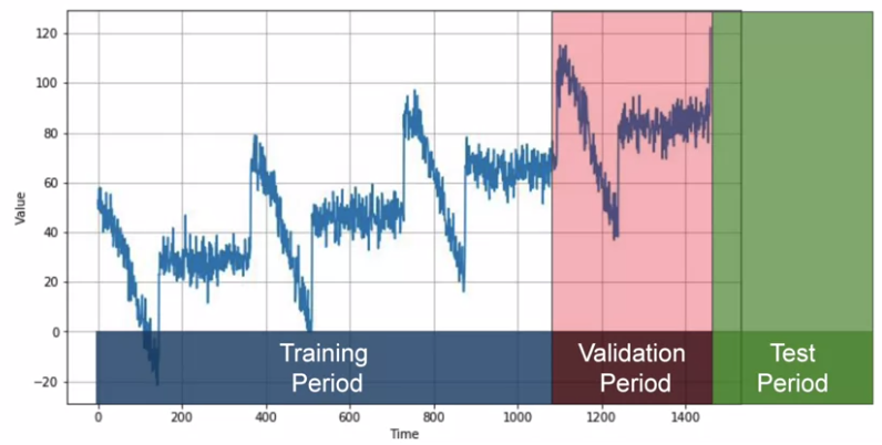
- Fixed partitioning (this course focuses on) = splitting TS data into training period, validation period and test period.
-
If TS is seasonal, we want each period contains the whole number of seasons.
-
-
We can split + train + test to get a model and then re-train with the data containing also the test period so that the model is optimized! In that case, the test set comes from the future.
-
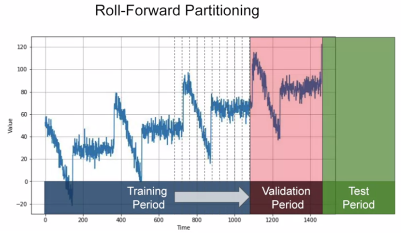
Roll-forward partitioning: we start with a short training period and we gradually increase it (1 day at a time or 1 week at a time). At each iteration, we train the model on training period, use it to focast the following day/week in the validation period. = Fixed partitioning in a number of times!
Metrics
For evaluating models:
errors = forecasts - actual

# Mean squared error (square to get rid of negative values)
# Eg. Used if large errors are potentially dangerous
mse = np.square(errors).mean()
# Get back to the same scale to error
rmse = np.sqrt(mse)

# Mean absolute error (his favorite)
# this doesn't penalize large errs as much as mse does,
# used if loss is proportional to the size of err
mae = np.abs(errors).mean()

# Mean abs percentage err
# idea of the size of err compared to the values
mape = np.abs(errors / x_valid).mean()
# MAE with TF
keras.metrics.mean_absolute_error(x_valid, naive_forecast).numpy()
Moving average and differencing
👉 Notebook: Forecasting. + explaining video.
Moving average: a simple forecasting method. Calculate the average of blue lines within a fixed “averaging windows”.
- This can eliminate noises and doesn’t anticipate trend or seasonality.
- Depend on the “averaging window”, it can give worse result than naive forecast.
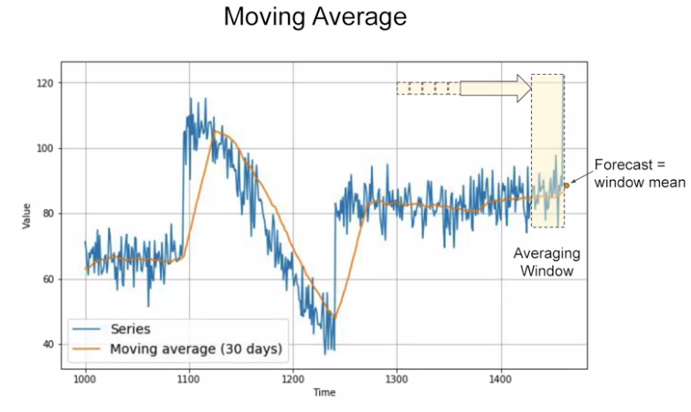 Take the average on each yellow window. MAE=7.14 (optimal is 4).
def moving_average_forecast(series, window_size):
    """Forecasts the mean of the last few values.
        If window_size=1, then this is equivalent to naive forecast"""
    forecast = []
    for time in range(len(series) - window_size):
    forecast.append(series[time:time + window_size].mean())
    return np.array(forecast)
Differencing: remove the trend and seasonality from the TS. We study on the differences between points and their previous neighbor in period.
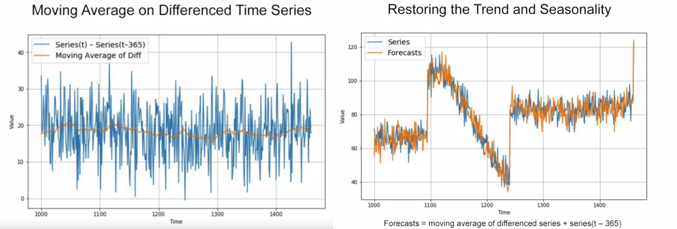 Left image: we find the differencing of original values, then we find the average (orange line). Right image: restore the trend and seasonality. MAE=5.8 (optimal is 4).
Above method still get the noises (because we add the differencing to the previous noise). If we remove past noise using moving average on that.
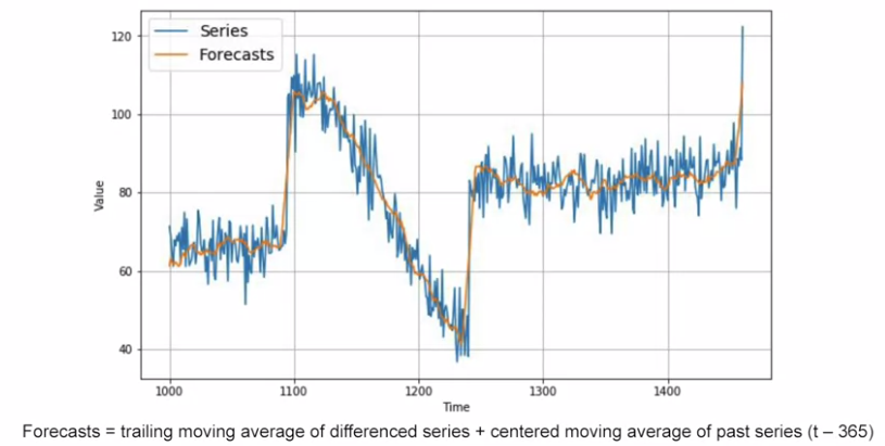 Smoothing both past and present values. MAE=4.5 (optimal is 4).
Keep in mind before using Deep Learning, sometimes simple approaches just work fine!
Deep NN for Time Series
Preparing features and labels
- We need to split our TS data into features and labels so that we can use them in ML algos.
- In this case: features=#values in TS, label=next_value.
- Feature: window size and train to predict next value.
- Ex: 30 days of values as features and next value as label.
- Overtime, train ML to match 30 features to match a single label.
👉 Notebook: Preparing features and labels.
👉 Video explains how to split to features and labels from dataset.
def windowed_dataset(series, window_size, batch_size, shuffle_buffer):
    dataset = tf.data.Dataset.from_tensor_slices(series)
    dataset = dataset.window(window_size + 1, shift=1, drop_remainder=True)
    dataset = dataset.flat_map(lambda window: window.batch(window_size + 1))
    dataset = dataset.shuffle(shuffle_buffer).map(lambda window: (window[:-1], window[-1]))
    dataset = dataset.batch(batch_size).prefetch(1)
    return dataset
Sequence bias
Sequence bias is when the order of things can impact the selection of things. It's ok to shuffle!
Feeding windowed datasets into NN
👉 Notebook: Single layer NN + video explains it.
# Simple linear regression (1 layer NN)
dataset = windowed_dataset(x_train, window_size, batch_size, shuffle_buffer_size)
l0 = tf.keras.layers.Dense(1, input_shape=[window_size])
model = tf.keras.models.Sequential([l0])
model.compile(loss="mse", optimizer=tf.keras.optimizers.SGD(lr=1e-6, momentum=0.9))
model.fit(dataset,epochs=100,verbose=0)
print("Layer weights {}".format(l0.get_weights()))

forecast = []

for time in range(len(series) - window_size):
    forecast.append(model.predict(series[time:time + window_size][np.newaxis]))
    # np.newaxis: reshape X to input dimension that used by the model

forecast = forecast[split_time-window_size:]
results = np.array(forecast)[:, 0, 0]
👉 Notebook: DNN with TS + video explains it.
# A way to choose an optimal learning rate
lr_schedule = tf.keras.callbacks.LearningRateScheduler(
    lambda epoch: 1e-8 * 10**(epoch / 20))
optimizer = tf.keras.optimizers.SGD(lr=1e-8, momentum=0.9)
model.compile(loss="mse", optimizer=optimizer)
history = model.fit(dataset, epochs=100, callbacks=[lr_schedule], verbose=0)
lrs = 1e-8 * (10 ** (np.arange(100) / 20))
plt.semilogx(lrs, history.history["loss"])
plt.axis([1e-8, 1e-3, 0, 300])
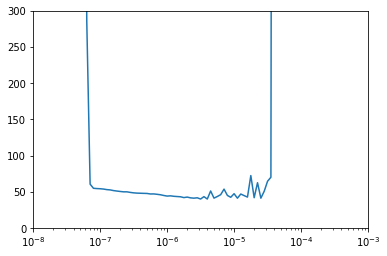 Loss w.r.t different learning rates. We choose the lowest one, around 8e-6.
👉 Notebook: DNN with synthetic TS.
RNN for TS
- RRN is a NN containing Recurrent layer.
- The different from DNN is the input shape is 3 dimensional (
batch_size x #time_step x dims_input_at each_timestep). - Re-use 1 cell multiple times in different layers (in this course).
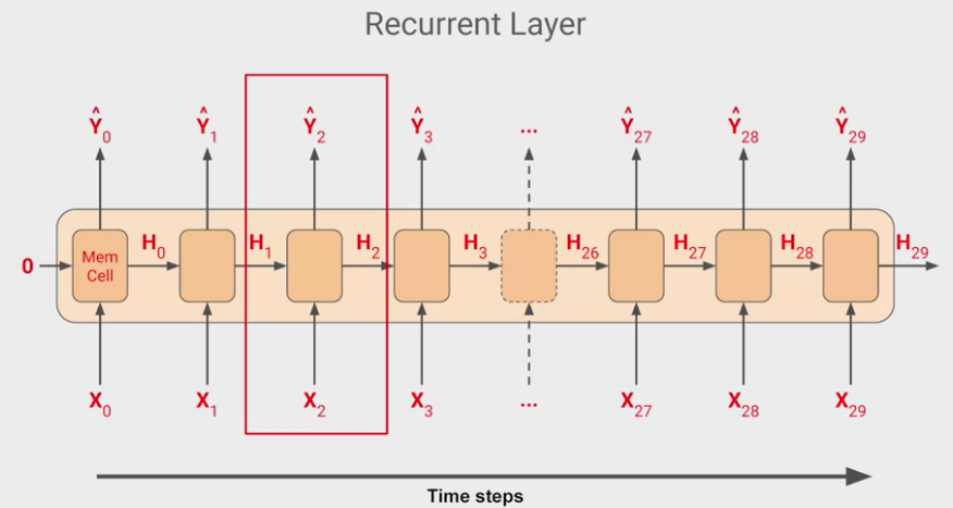 Idea of how RNN works with TS data. The current location can be impacted more by the nearby locations.
Shape of input to RNN
👉 Video explains the dimensional and sequence-to-vector RNN.
- Suppose: window size of 30 time steps, batch size of 4: Shape will be 4x30x1 and the memory cell input will be 4x1 matrix.
- If the memory cell comprises 3 neurons then the output matrix will be 4x3. Therefore, the full output of the layer will be 4x30x3.
- is just a copy of .
- Below figure: input and also output a sequence.
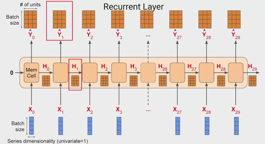 Dimension of input to RNN.
Sequence to vector RNN
- Sometimes, we want only input a sequence but not output. This called sequence-to-vector RNN. I.E., ignore all of the outputs except the last one!. In
tf.keras, it’s default setting!
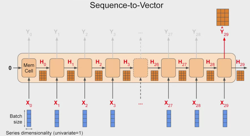 Sequence to vector RNN.
# Check the figure below as an illustration
model = tf.keras.models.Sequential([
tf.keras.layers.SimpleRNN(20, return_sequences=True, input_shape=[None, 1]),
    # input_shape:
    #   TF assumes that 1st dim is batch size -> any size at all -> no need to define
    #   None -> number of time steps, None means RNN can handle sequence of any length
    #   1 -> univariate TS
tf.keras.layers.SimpleRNN(20),
    # if there is `return_sequences=True` -> sequence-to-sequence RNN
tf.keras.layers.Dense(1),
])
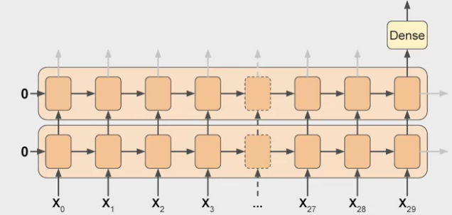 Illustration with keras.
Lambda layer
👉 Video explains the use of lambda layer in RNN..
model = tf.keras.models.Sequential([
    tf.keras.layers.Lambda(lambda x: tf.expand_dims(x, axis=-1), # expand to 1 dim (from 2) so that we have 3 dims: batch size x #timesteps x series dim
                        input_shape=[None]), # can use any size of sequences
    tf.keras.layers.SimpleRNN(40, return_sequences=True),
    tf.keras.layers.SimpleRNN(40),
    tf.keras.layers.Dense(1),
    tf.keras.layers.Lambda(lambda x: x * 100.0)
        # default activation in RNN is tanh -> (-1, 1) -> scale to -100, 100
])
Simple RNN
- Loss function Huber (wiki): less sensitive to outliers. => we use this because our data in this case get a little bit noisy!
👉 Notebook: Simple RNN with a TS data + videos explains it.
LSTM
👉 Notebook: LSTM with a TS data + videos explains it.
# clear internal variables
tf.keras.backend.clear_session()
dataset = windowed_dataset(x_train, window_size, batch_size, shuffle_buffer_size)

model = tf.keras.models.Sequential([
    tf.keras.layers.Lambda(lambda x: tf.expand_dims(x, axis=-1),
                        input_shape=[None]),
    # LSTM here
    tf.keras.layers.Bidirectional(tf.keras.layers.LSTM(32, return_sequences=True)),
    tf.keras.layers.Bidirectional(tf.keras.layers.LSTM(32, return_sequences=True)),
    tf.keras.layers.Bidirectional(tf.keras.layers.LSTM(32)),
    #
    tf.keras.layers.Dense(1),
    tf.keras.layers.Lambda(lambda x: x * 100.0)
])
👉 Notebook: LSTM with synthetic TS.
Real-world time series data
- We are going to predict the sunspot actitivity cycles (download dataset).
- Combine CNN + LSTM.
👉 Andrew’s video on Optimization Algo: Mini-batch gradient descent.
👉 Notebook: Sunspot dataset with CNN+LSTM. + video explains it.
👉 Notebook: Sunspot dataset with DNN only + explaining video.
👉 Video explains train & tune the model (how to choose suitable values for sizes)
