Last modified on 01 Oct 2021.
This is my note for the first course of TensorFlow in Practice Specialization given by deeplearning.ai and taught by Laurence Moroney on Coursera.
👉 Check the codes on my Github.
👉 Official notebooks on Github.
👉 Go to course 2 - CNN in Tensorflow.
👉 Go to course 3 - NLP in Tensorflow.
👉 Go to course 4 - Sequences, Time Series and Prediction.
Basic DL on MNIST
import tensorflow as tf

# stop the training with condition
class myCallback(tf.keras.callbacks.Callback):
    def on_epoch_end(self, epoch, logs={}): # compare at the end of each epoch
        if(logs.get('accuracy') > 0.99):
            self.model.stop_training = True

mnist = tf.keras.datasets.mnist
(x_train, y_train),(x_test, y_test) = mnist.load_data()
x_train, x_test = x_train / 255.0, x_test / 255.0 # normalize

callbacks = myCallback() # define the callback

model = tf.keras.models.Sequential([
    tf.keras.layers.Flatten(input_shape=(28, 28)), # Takes that square and
                                                   # turns it into a 1 dim
    tf.keras.layers.Dense(512, activation=tf.nn.relu),
    tf.keras.layers.Dense(10, activation=tf.nn.softmax) # 10 outputs
])

model.compile(optimizer='adam',
              loss='sparse_categorical_crossentropy',
              metrics=['accuracy'])

model.fit(x_train, y_train, epochs=10, callbacks=[callbacks])
Comments (notebook):
- Adding more Neurons we have to do more calculations, slowing down the process, but get more accurate.
- The first layer in your network should be the same shape as your data.
- The number of neurons in the last layer should match the number of classes you are classifying for.
- Extra layers are often necessary.
- Flatten as the name implies, converts your multidimensional matrices (
Batch.Size x Img.W x Img.H x Kernel.Size) to a nice single 2-dimensional matrix: (Batch.Size x (Img.W x Img.H x Kernel.Size)). During backpropagation it also converts back your delta of size (Batch.Size x (Img.W x Img.H x Kernel.Size)) to the original (Batch.Size x Img.W x Img.H x Kernel.Size). - Dense layer is of course the standard fully connected layer.
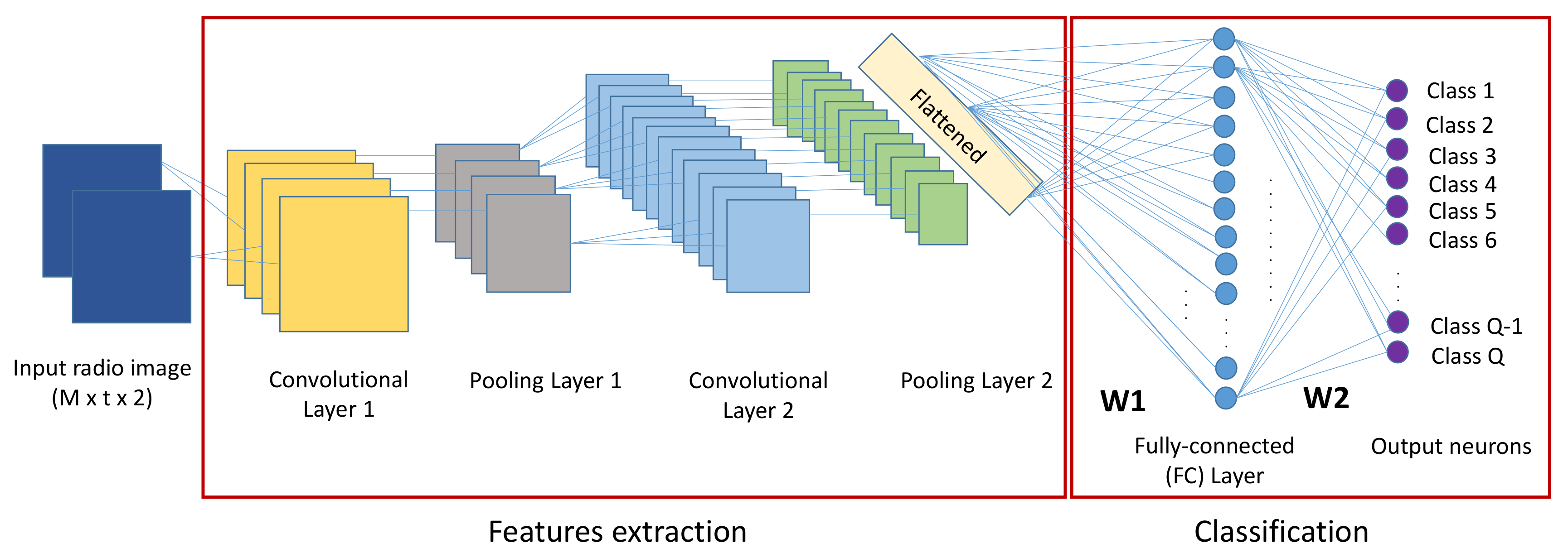
 CNN layers, cource of image.
Basic DL on Fashion-MNIST
# the same as in MINST
# different at below line of loading data
mnist = tf.keras.datasets.fashion_mnist
Basic CNN on Fashion-MNIST
import tensorflow as tf
mnist = tf.keras.datasets.fashion_mnist

class myCallback(tf.keras.callbacks.Callback):
    def on_epoch_end(self, epochs, logs={}) :
        if(logs.get('accuracy') is not None and logs.get('accuracy') >= 0.998) :
            print('\nReached 99.8% accuracy so cancelling training!')
            self.model.stop_training = True

(training_images, training_labels), (test_images, test_labels) = mnist.load_data()
# Why reshape?
# The first convolution expects a single tensor containing everything,
# so instead of 60000 28x28x1 items in a list, we have a single 4D list
# that is 60000x28x28x1
#
# training_images' shape (before reshape): (60000, 28, 28)
# training_images' shape (after reshape): (60000, 28, 28, 1)
# trainaing_labels' shape: (60000,)
training_images=training_images.reshape(60000, 28, 28, 1)
training_images=training_images / 255.0
test_images = test_images.reshape(10000, 28, 28, 1)
test_images=test_images/255.0

model = tf.keras.models.Sequential([
  tf.keras.layers.Conv2D(64, (3,3), activation='relu', input_shape=(28, 28, 1)),
  tf.keras.layers.MaxPooling2D(2, 2),
  tf.keras.layers.Conv2D(64, (3,3), activation='relu'),
  tf.keras.layers.MaxPooling2D(2,2),
  tf.keras.layers.Flatten(),
  tf.keras.layers.Dense(128, activation='relu'),
  tf.keras.layers.Dense(10, activation='softmax')
])

model.compile(optimizer='adam',
              loss='sparse_categorical_crossentropy',
              metrics=['accuracy'])

callbacks = myCallback()

model.fit(training_images, training_labels, epochs=5, callbacks=[callbacks])
test_loss = model.evaluate(test_images, test_labels)
model.summary() # model detail
Model: "sequential_1"
_________________________________________________________________
Layer (type)                 Output Shape              Param #
=================================================================
conv2d (Conv2D)              (None, 26, 26, 64)        640
                             # for every image, 64 convolution has been tried
                             # 26 (=28-2) because we use 3x3 filter and we can't
                             # count on edges, so the picture is 2 smaller on x and y.
                             # if 5x5 filter => 4 smaller on x and y.
_________________________________________________________________
max_pooling2d (MaxPooling2D) (None, 13, 13, 64)        0
_________________________________________________________________
conv2d_1 (Conv2D)            (None, 11, 11, 64)        36928
_________________________________________________________________
max_pooling2d_1 (MaxPooling2 (None, 5, 5, 64)          0
_________________________________________________________________
flatten_1 (Flatten)          (None, 1600)              0
_________________________________________________________________
dense_2 (Dense)              (None, 128)               204928
_________________________________________________________________
dense_3 (Dense)              (None, 10)                1290
=================================================================
Total params: 243,786
Trainable params: 243,786
Non-trainable params: 0
Refs:
- Kernel in image processing: examples with images.
- Pooling layer: non-linear down-sampling.
More?
- Image Filtering – Lode’s Computer Graphics Tutorial
- Applying Convolutions on top of our Deep neural network will make training => It depends on many factors. It might make your training faster or slower, and a poorly designed Convolutional layer may even be less efficient than a plain DNN!
- What is a Convolution? => A technique to isolate features in images
- What is a Pooling? => A technique to reduce the information in an image while maintaining features
- How do Convolutions improve image recognition? => They isolate features in images
-
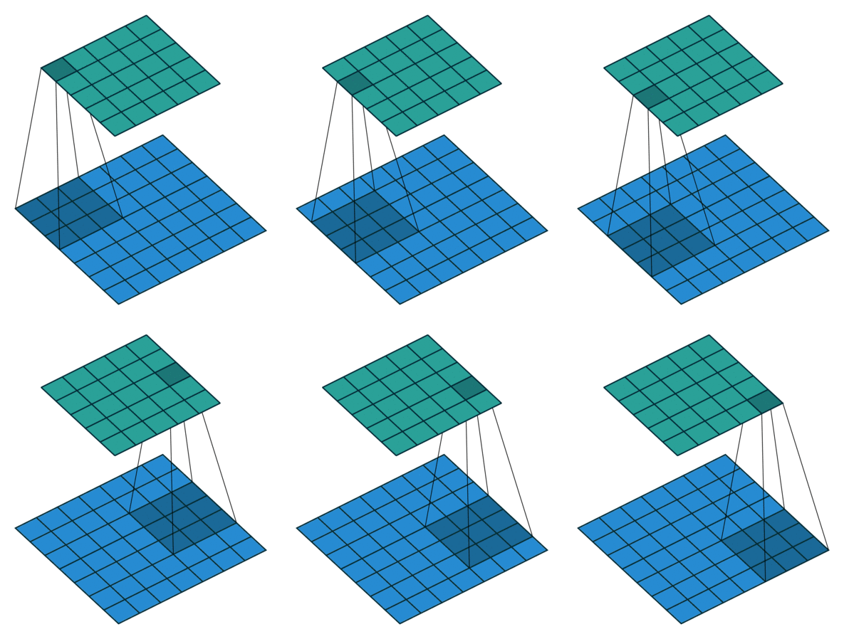
After passing a 3x3 conv filter over a 28x28 image, how big will the output be? => 26x26
 7x7 to 5x5 (source)
 -
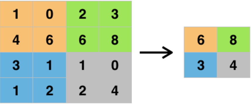
After max pooling a 26x26 image with a 2x2 filter, how big will the output be? => 13x13
 (source)
Visualizing the Convolutions and Pooling
Using layer API, something like below, check more in the notebook.
import matplotlib.pyplot as plt
f, axarr = plt.subplots()

from tensorflow.keras import models
layer_outputs = [layer.output for layer in model.layers]
activation_model = tf.keras.models.Model(inputs = model.input, outputs = layer_outputs)

for x in range(0,4):
    f1 = activation_model.predict(test_images[FIRST_IMAGE].reshape(1, 28, 28, 1))[x]
    axarr[0,x].imshow(f1[0, : , :, CONVOLUTION_NUMBER], cmap='inferno')
    axarr[0,x].grid(False)
    ...
Using real-world images
An example of classifying horses and humans!
ImageGenerator
👉 Video explain ImageGenerator.
# make images more used for training
# (focus on object, split cleary objects, label images,...)
# also help to augmenting data (rotate, skew, flip,...)
from tensorflow.keras.preprocessing.image import ImageDataGenerator

train_datagen = ImageDataGenerator(rescale=1./255)
    # normalize -> No need to convert images and then put in the training
    # do the scaling on the fly
train_generator = train_datagen.flow_from_directory(
    train_dir, # dir contains the dir containing your images
               # -> be careful!
    target_size=(300, 300), # images will be resized when loaded, genial!
                            # because NN always needs that!
                            # -> experimenting with diff sizes without
                            # impacting your source data
    batch_size=128,
    class_mode="binary"     # 2 diff things
)

test_datagen = ImageDataGenerator(rescale=1./255) # normalize
validation_generator = test_datagen.flow_from_directory(
    validation_dir, # dir contains the dir containing your images
    target_size=(300, 300),
    batch_size=32,
    class_mode="binary"
)
ConvNet with ImageGenerator
More docs:
- Understanding Categorical Cross-Entropy Loss, Binary Cross-Entropy Loss, Softmax Loss, Logistic Loss, Focal Loss and all those confusing names
- Overview of mini-batch gradient descent
