Principal Component Analysis (PCA)

Last modified on 01 Oct 2021.

What?

Sometimes we need to “compress” our data to speed up algorithms or to visualize data. One way is to use dimensionality reduction which is the process of reducing the number of random variables under consideration by obtaining a set of principal variables. We can think of 2 approaches:

• Feature selection: find a subset of the input variables.
• Feature projection (also Feature extraction): transforms the data in the high-dimensional space to a space of fewer dimensions. PCA is one of the methods following this approach.

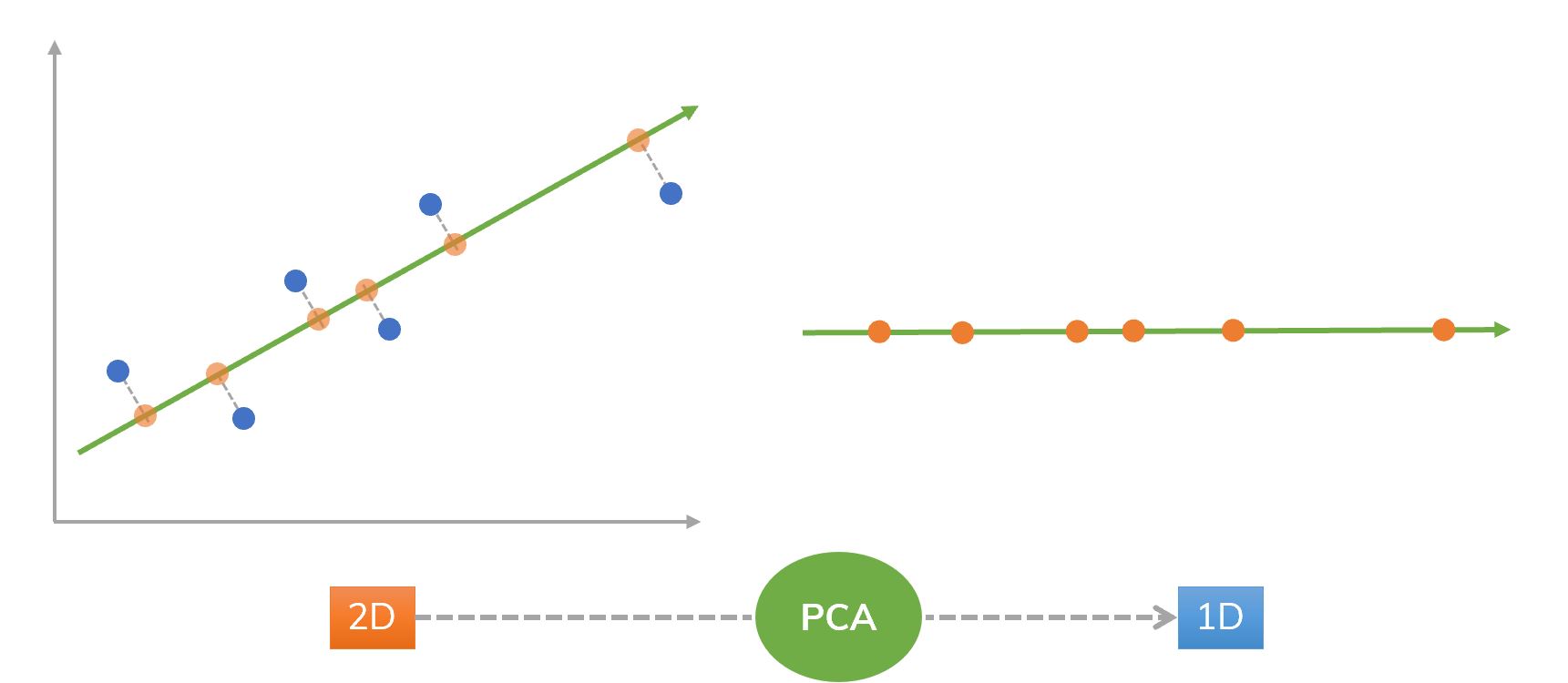Figure 1. An idea of using PCA from 2D to 1D.

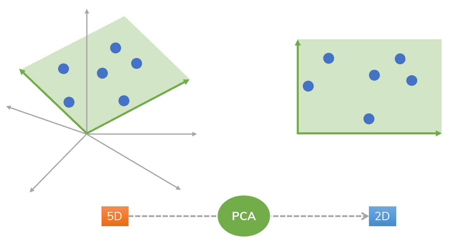Figure 2. An idea of using PCA from 5D to 2D.

❓ Questions: How can we choose the green arrows like in Figure 1 and 2 (their directions and their magnitudes)?

From a data points, there are many ways of projections, for examples,

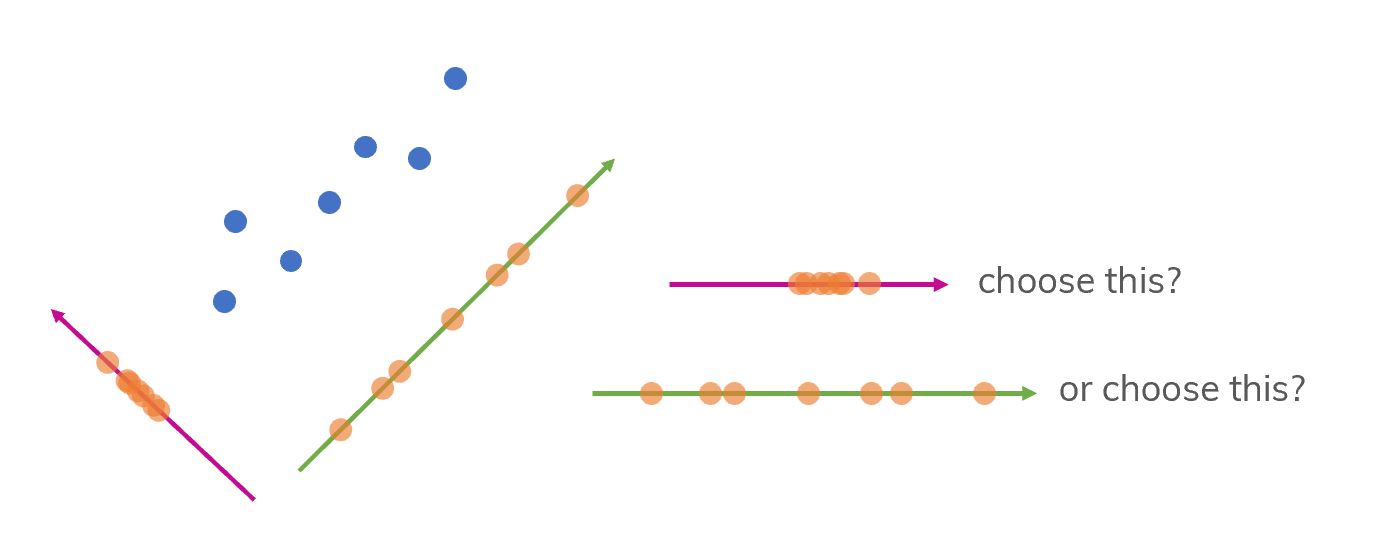Figure 3. We will project the points to the green line or the violet line? Which one is the best choice?

Intuitively, the green line is better with more separated points. But how can we choose it “mathematically” (precisely)? We need to know about:

• Mean: find the most balanced point in the data.
• Variance: measure the spread of data from the mean. However, variance is not enough. There are many different ways in that we get the same variance.
• Covariance: indicate the direction in that data are spreading.

An example of the same mean and variance but different covariance.

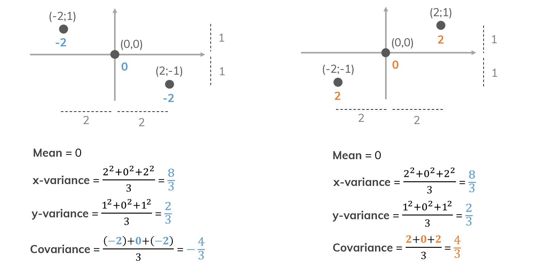Figure 4. Different data but the same mean and variance. That’s why we need covariance!

Algorithm

1. Subtract the mean to move to the original axes.
2. From the original data (a lot of features $x_1, x_2, \ldots, x_N$), we construct a covariance matrix $U$.
3. Find the eigenvalues $\lambda_1, \lambda_2,\ldots$ and correspondent eigenvectors $v_1, v_2, \ldots$ of that matrix (we call them eigenstuffs). Choose $K < N$ couples $\lambda$ and $v$ (the highest eigenvalues) and we get a reduced matrix $U_K$.

4. Projection original data points to the $K$-dimensional plane created based on these new eigenstuffs. This step creates new data points on a new dimensional space ($K$).

   $Z = U_K^TX$

5. Now, instead of solving the original problem ($N$ features), we only need to solve a new problem with $K$ features ($K<N$).

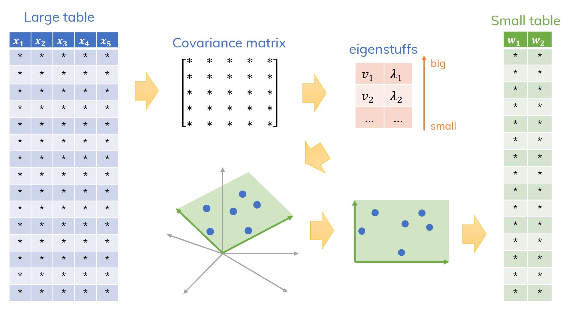Figure 5. A big picture of the idea of PCA algorithm.^[ref]

Code

from sklearn.decomposition import PCA

s = np.array([...])
pca = PCA(n_components=150, whiten=True, random_state=42)
# pca.fit(s)
s1 = pca.fit_transform(s)

print (pca.components_) # eigenvectors
print (pca.explained_variance_) # eigenvalues

Some notable components (see full):

• pca.fit(X): only fit X (and then we can use pca for other operations).
• pca.fit_transform(X): Fit the model with X and apply the dimensionality reduction on X (from (n_samples, n_features) to (n_samples, n_components)).
• pca.inverse_transform(s1): transform s1 back to original data space (2D) - not back to s!!!
• pca1.mean_: mean point of the data.
• pca.components_: eigenvectors (n_components vectors).
• pca.explained_variance_: eigenvalues. It’s also the amount of retained variance which is corresponding to each components.
• pca.explained_variance_ratio_: the percentage in that variance is retained if we consider on each component.

Some notable parameters:

• n_components=0.80: means it will return the Eigenvectors that have the 80% of the variation in the dataset.

[0.32047581  0.59549787  0.80178824  0.932976    1.]

Whitening

Whitening makes the features:

• less correlated with each other,
• all features have the same variance (or, unit component-wise variances).

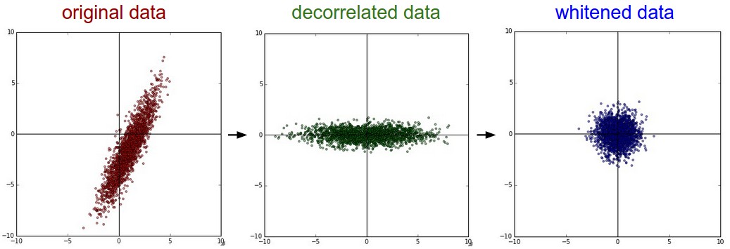PCA / Whitening. Left: Original toy, 2-dimensional input data. Middle: After performing PCA. The data is centered at zero and then rotated into the eigenbasis of the data covariance matrix. This decorrelates the data (the covariance matrix becomes diagonal). Right: Each dimension is additionally scaled by the eigenvalues, transforming the data covariance matrix into the identity matrix. Geometrically, this corresponds to stretching and squeezing the data into an isotropic gaussian blob.

If this section doesn’t satisfy you, read this and this (section PCA and Whitening).

PCA in action

• Example to understand the idea of PCA: –

  • Plot points with 2 lines which are corresponding to 2 eigenvectors.
  • Plot & choose Principal Components.
  • An example of choosing n_components $K$.
  • Visualization hand-written digits (the case of all digits and the case of only 2 digits – 1 & 8).
  • Using SVM to classifier data in the case of 1 & 8 and visualize the decision boundaries.

• Image compression: –

  • When input is an image, the values of adjacent pixels are highly correlated.
  • Import images from scipy and Google Drive or Github (with git).
  • Compress grayscale images and colored ones.
  • Plot a grayscale version of a colorful images.
  • Save output to file (Google Drive).
  • Fix warning Lossy conversion from float64 to uint8. Range […,…]. Convert image to uint8 prior to saving to suppress this warning.
  • Fix warning Clipping input data to the valid range for imshow with RGB data ([0..1] for floats or [0..255] for integers).
  • Calculate a size (in KB) of a image file.

• PCA without scikit-learn: –

References

• Luis Serrano – [Video] Principal Component Analysis (PCA). It’s very intuitive!
• Stats.StackExchange – Making sense of principal component analysis, eigenvectors & eigenvalues.
• Scikit-learn – PCA official doc.
• Tiep Vu – Principal Component Analysis: Bài 27 and Bài 28.
• Jake VanderPlas – In Depth: Principal Component Analysis.
• Tutorial 4 Yang – Principal Components Analysis.
• Andrew NG. – My raw note of the course “Machine Learning” on Coursera.
• Shankar Muthuswamy – Facial Image Compression and Reconstruction with PCA.
• UFLDL - Stanford – PCA Whitening.

×Close