Last modified on 01 Oct 2021.

What’s the idea of SVM?

SVM (also called Maximum Margin Classifier) is an algorithm that takes the data as an input and outputs a line/hyperplane that separates those classes if possible.

Suppose that we need to separate two classes of a dataset. The task is to find a line to separate them. However, there are many lines which can do that (countless number of lines). How can we choose the best one?
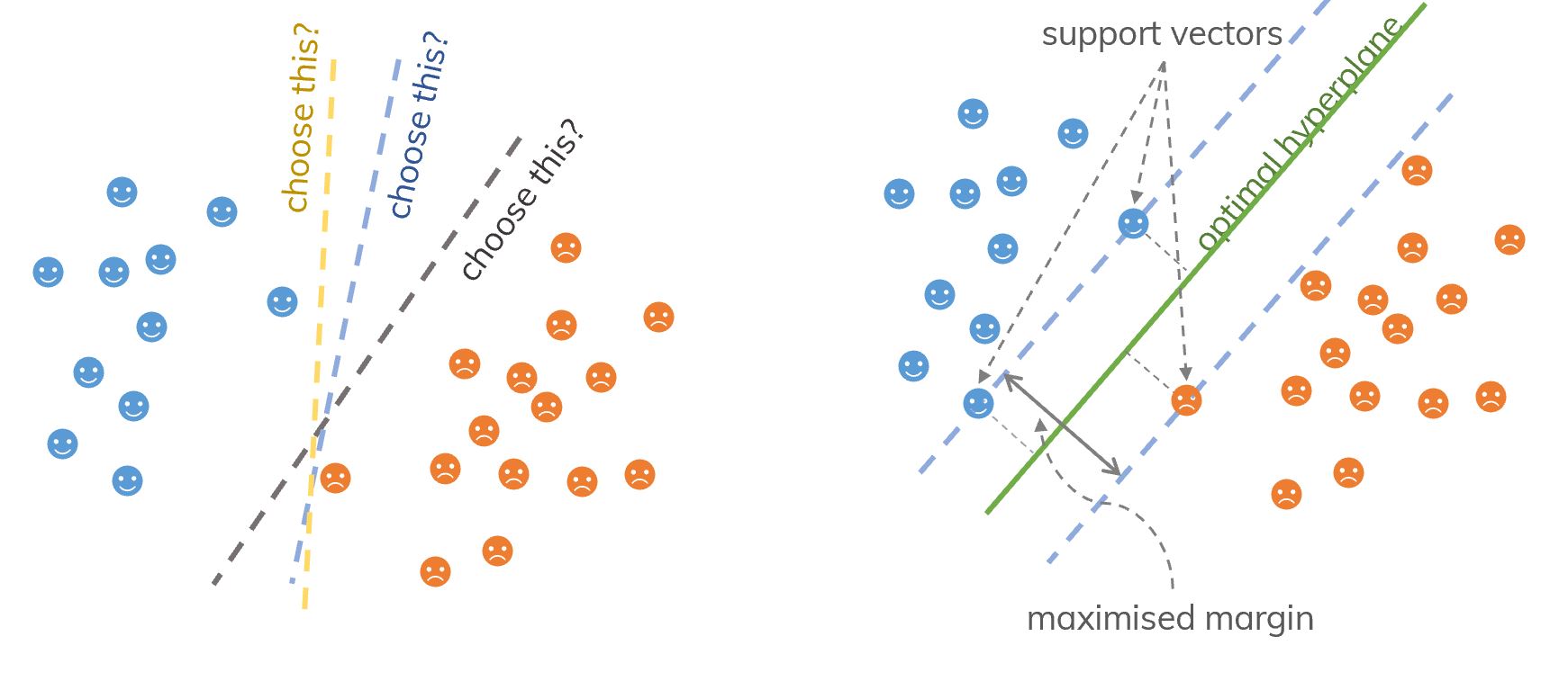
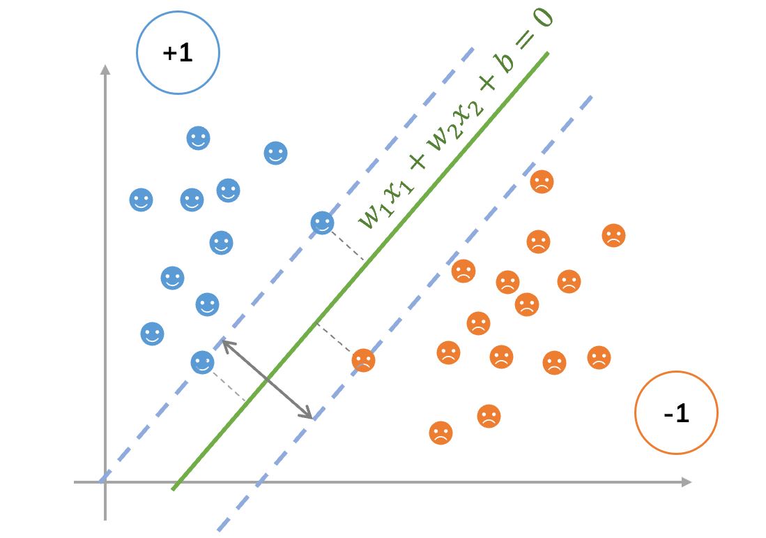
An idea of support vectors and SVM. An idea of support vectors (samples on the margin) and SVM (find the optimal hyperplane).

We need to find a hyperplane (H)(H): wTx+b=0\mathbf{w}^T\mathbf{x} + b = 0 where the weights w=(w1,,wd)\mathbf{w}=(w_1,\ldots,w_d) and a point x=(x1,,xd)\mathbf{x}=(x_1,\ldots,x_d). For example, in 2D (d=2d=2), we need to find a hyperplane w1x1+w2x2+b=0w_1x_1 + w_2x_2 + b=0. Note also that, the distance between a point x0\mathbf{x}_0 and (H)(H) is given by,

d(x0,H)=wTx0+bw2,(1) \text{d}(\mathbf{x}_0, H) = \frac{\vert\mathbf{w}^T\mathbf{x}_0 + b\vert}{\Vert\mathbf{w}\Vert_2}, \quad (1)

where w2=i=1dwi2\Vert\mathbf{w}\Vert_2 = \sqrt{\sum_{i=1}^d w_i^2}.

In order to understand the idea, we consider a 2D case with the classification of 2 classes (blue faces are numbered as “+1+1” and orange faces are numbered as “1-1”).

Finding a hyperplane. We need to find an optimal hyperplane between 2 classes (find w1,w2w_1, w_2 and bb).

Recall that a margin (geometric margin) is the minimum distance between a hyperplane and the closest point(s) to it. Thanks to (1)(1), we can find the margin to a hyperplane by determining the closet distance from an arbitrary points (xi,yi)(\mathbf{x}_i, y_i) to that hyperplane via,

margin=miniyi(wTxi+b)w2.(2) \text{margin} = \min_i \frac{y_i(\mathbf{w}^T\mathbf{x}_i + b)}{||\mathbf{w}||_2}. \quad (2)

Note that, because yiy_i takes values 1-1 or +1+1 and it always has the same sign as wTxi+b\mathbf{w}^T\mathbf{x}_i + b, yi(wTxi+b)y_i(\mathbf{w}^T\mathbf{x}_i + b) is always positive.

The SVM problem is to find (w,b\mathbf{w}, b) so that the hard-margin (2)(2) has the maximum value, i.e.,

(w,b)=argmaxw,b(miniyi(wTxi+b)w2)=argmaxw,b(1w2miniyi(wTxi+b))(3) \begin{aligned} (\mathbf{w}, b) &= \arg \max_{\mathbf{w}, b} \left( \min_i \frac{y_i(\mathbf{w}^T\mathbf{x}_i + b)}{\Vert\mathbf{w}\Vert_2} \right)\\ &= \arg \max_{\mathbf{w}, b}\left( \frac{1}{\Vert\mathbf{w}\Vert_2} \min_i y_i(\mathbf{w}^T\mathbf{x}_i + b) \right) \end{aligned} \quad (3)

(arg\arg means you need to find w,b\mathbf{w},b so that the function reaches the max\max.)

This is an optimal problem. Another remark is that we can multiply both sides of (H)(H) by any real number k0k\ne 0, we obtain the same (H)(H). With that reason, we can suppose that,

yi(wTxi+b)=1, y_i(\mathbf{w}^T\mathbf{x}_i + b) = 1,

for all points on the hyperplane, and the problem (3)(3) becomes,

(w,b)=argmaxw,b1w2subject to  yi(wTxi+b)1,i=1,2,,N. \begin{aligned} &(\mathbf{w}, b) = \arg\max_{\mathbf{w}, b} \frac{1}{\Vert\mathbf{w}\Vert_2} \\ \text{subject to} &~~ y_i(\mathbf{w}^T\mathbf{x}_i + b) \geq 1, \forall i = 1, 2, \dots, N. \end{aligned}

The second line due to the fact that the closet points have distance 11 to the hyperplane, the other points have distance greater than 11. We can write above problem as,

(w,b)=argminw,b12w22subject to  yi(wTxi+b)10,i=1,2,,N.(4) \begin{aligned} &(\mathbf{w}, b) = \arg\min_{\mathbf{w}, b} \frac{1}{2}\Vert\mathbf{w}\Vert_2^2 \\ \text{subject to} &~~ y_i(\mathbf{w}^T\mathbf{x}_i + b)-1 \geq 0, \forall i = 1, 2, \dots, N. \end{aligned} \quad (4)

This is called “primal formulation of linear SVMs”. In mathematical optimization, one can prove that the problem (4)(4) has an unique solution (We can get an unique hyperplane (H)(H) which satisfies the classification problem). Such problems are generally called quadratic programming problems.

Problem (4)(4) can be solved “more easily” by considering its dual formulation. Apply the method of Lagrange multipliers, we define a Lagrangian,

Λ(w,b,λ)=12w22i=1Nλi(yi(wTxi+b)1), \Lambda(\mathbf{w},b,\lambda) = \dfrac{1}{2}\Vert \mathbf{w}\Vert_2^2 - \sum_{i=1}^N \lambda_i(y_i(\mathbf{w}^T\mathbf{x}_i+b)-1),

where w,xi\mathbf{w}, \mathbf{x}_i are vectors with dd elements and λ\lambda is a vector with NN elements. We need to minimize this Lagrangian w.r.t. w,b\mathbf{w}, b and simultaneously require that the derivative w.r.t. λ\lambda vanishes, all subject to the constraints that λi0\lambda_i \ge 0. If we set the derivatives w.r.t. w,b\mathbf{w}, b, we obtain,

Λ(w,b,λ)b=0i=1Nλiyi=0,Λ(w,b,λ)w=0w=i=1Nλiyixi. \begin{aligned} \dfrac{\partial \Lambda(\mathbf{w},b,\lambda)}{\partial b} &= 0 \Rightarrow \sum_{i=1}^N\lambda_iy_i=0, \\ \dfrac{\partial \Lambda(\mathbf{w},b,\lambda)}{\partial \mathbf{w}} &= 0 \Rightarrow \mathbf{w}=\sum_{i=1}^N\lambda_iy_i\mathbf{x}_i. \end{aligned}

We substitute the above into the equation for Γ(w,b,λ)\Gamma(\mathbf{w},b,\lambda) and obtain “dual formulation of linear SVMs”,

λ=argmaxλ(i=1Nλi12i=1Nj=1NλiλjyiyjxiTxj)subject to  λi0,i=1Nλiyi=0, i=1,,N.(5) \begin{aligned} &\lambda = \arg\max_{\lambda} \left( \sum_{i=1}^N \lambda_i -\frac{1}{2}\sum_{i=1}^N \sum_{j=1}^N \lambda_i\lambda_j y_i y_j \mathbf{x}_i^T\mathbf{x}_j \right) \\ \text{subject to} &~~ \lambda_i \ge 0, \sum_{i=1}^N\lambda_iy_i = 0, ~\forall i=1,\ldots,N. \end{aligned} \quad (5)

in that, w\mathbf{w} is defined in terms of λi\lambda_i: w=1Nλiyixi\mathbf{w} = \sum_1^N\lambda_iy_i\mathbf{x}_i and the solution becomes

f(x)=sign(Σ1NλiyixiTxj+b). f(\mathbf{x})=\text{sign}(\Sigma_1^N\lambda_iy_i\mathbf{x}_i^T\mathbf{x}_j + b).

Then given a new instance x\mathbf{x}, the classifier is,

f(x)=sign(wTx+b). f(\mathbf{x})=\text{sign}(\mathbf{w}^T\mathbf{x} + b).

The benefits of using dual formulation are:[ref, slide 52]

  • No need to access original data, need to access only dot products xiTxj\mathbf{x}_i^T\mathbf{x}_j.
  • Number of free parameters is bounded by the number of support vectors and not by the number of variables (beneficial for high-dimensional problems).

Read more in this post (Vietnamese), this slide or this post.

Using SVM with kernel trick

Most of the time, we cannot separate classes in the current dataset easily (not linearly separable data). We need to use kernel trick first (transform from the current dimension to a higher dimension) and then we use SVM. These classes are not linearly separable.
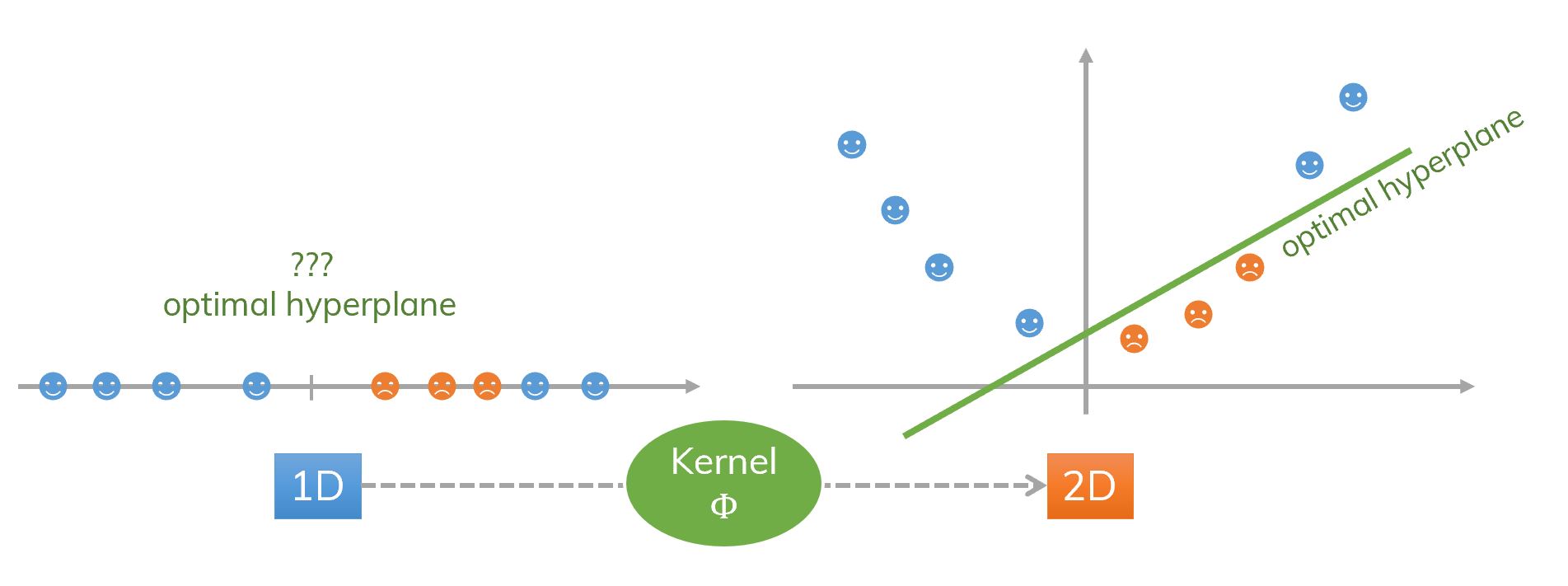
An idea of kernel and SVM (1D to 2D). An idea of kernel and SVM. Transform from 1D to 2D. Data is not linearly separable in the input space but it is linearly separable in the feature space obtained by a kernel.
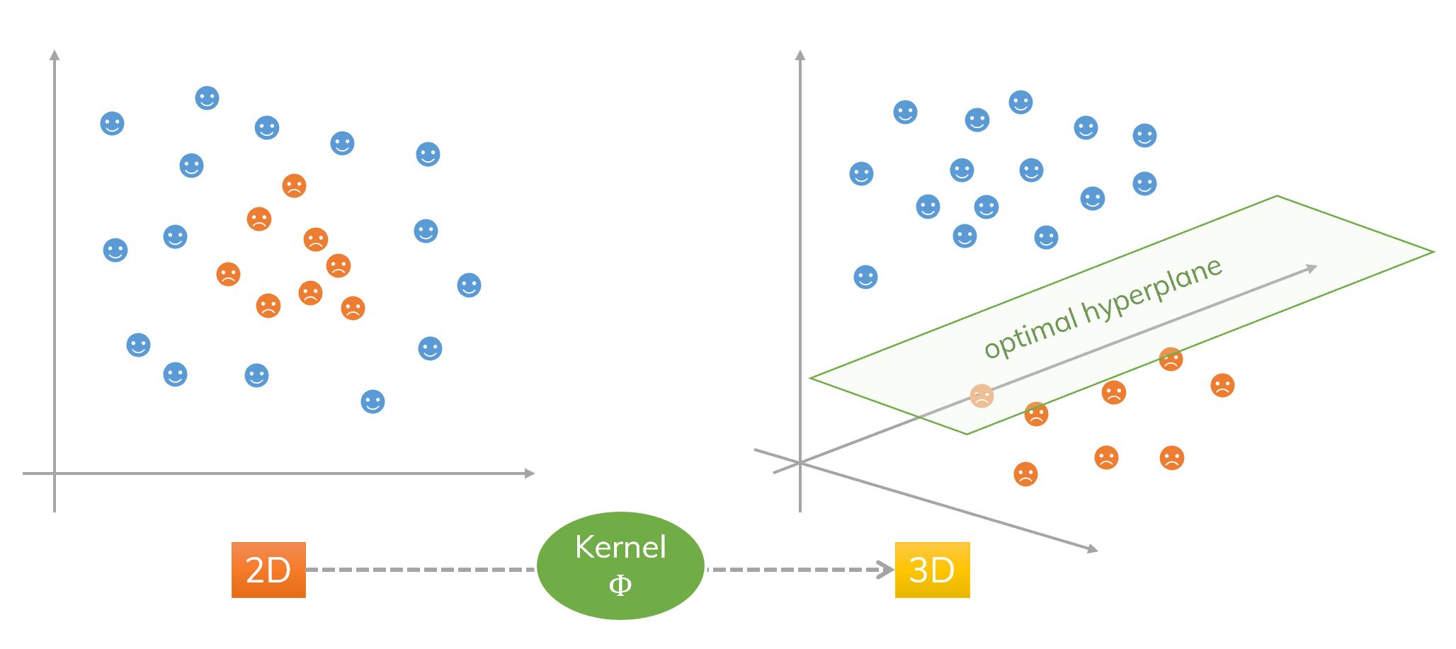
An idea of kernel and SVM (2D to 3D). An idea of kernel and SVM. Transform from 2D to 3D. Data is not linearly separable in the input space but it is linearly separable in the feature space obtained by a kernel.

Original data x\mathbf{x} (in input space),

f(x)=sign(wTx+b),w=i=1Nλiyixi \begin{aligned} f(\mathbf{x}) =\text{sign}(\mathbf{w}^T\mathbf{x} + b), \quad \mathbf{w} =\sum_{i=1}^N\lambda_iy_i\mathbf{x}_i \end{aligned}

Data in a higher dimensional feature space Φ(x)\Phi(\mathbf{x}),

f(x)=sign(wTΦ(x)+b),w=i=1NλiyiΦ(xi) \begin{aligned} f(\mathbf{x}) =\text{sign}(\mathbf{w}^T\Phi(\mathbf{x}) + b), \quad \mathbf{w} =\sum_{i=1}^N\lambda_iy_i\Phi(\mathbf{x}_i) \end{aligned}

We can rewrite f(x)f(\mathbf{x}) as,

f(x)=sign(i=1NλiyiΦ(xi)TΦ(x)+b), f(\mathbf{x}) =\text{sign} \left( \sum_{i=1}^N\lambda_iy_i\Phi(\mathbf{x}_i)^T\Phi(\mathbf{x}) + b \right),

or,

f(x)=sign(i=1NλiyiK(xi,x)+b),K(xi,x)=Φ(xi)TΦ(x). \begin{aligned} f(\mathbf{x}) &=\text{sign}(\sum_{i=1}^N\lambda_iy_iK(\mathbf{x}_i,\mathbf{x}) + b), \\ K(\mathbf{x}_i,\mathbf{x}) &= \Phi(\mathbf{x}_i)^T\Phi(\mathbf{x}). \end{aligned}

Therefore, we do not need to know Φ\Phi explicitly, we just need to define a kernel function K(,):Rd×RdRK(\cdot,\cdot): \mathbb{R}^d\times \mathbb{R}^d \to \mathbb{R}. However, not every function Rd×RdR\mathbb{R}^d\times \mathbb{R}^d \to \mathbb{R} can be a valid kernel. It has to satisfy so-called Mercer conditions. Otherwise, the underlying quadratic program may not be solvable.

A kernel is a dot product in some feature space:

K(xi,xj)=Φ(xi,xj). K(\mathbf{x}_i, \mathbf{x}_j) = \Phi(\mathbf{x}_i, \mathbf{x}_j).

It also measures the similarity between two points xi\mathbf{x}_i and xj\mathbf{x}_j.

We have some popular kernels,

  • Linear kernel: K(xi,xj)=xixjK(\mathbf{x}_i, \mathbf{x}_j) = \mathbf{x}_i \cdot \mathbf{x}_j. We use kernel = 'linear' in sklearn.svm.SVM. Linear kernels are rarely used in practice.
  • Gaussian kernel (or Radial Basic Function – RBF): K(xi,xj)=exp(γxixj2)K(\mathbf{x}_i, \mathbf{x}_j) = \exp(-\gamma\Vert \mathbf{x}_i - \mathbf{x}_j \Vert^2). It’s used the most. We use kernel = 'rbf' (default) with keyword gamma for γ\gamma (must be greater than 00) in sklearn.svm.SVM.
  • Exponential kernel: K(xi,xj)=exp(γxixj)K(\mathbf{x}_i, \mathbf{x}_j) = \exp(-\gamma\Vert \mathbf{x}_i - \mathbf{x}_j \Vert).
  • Polynomial kernel: K(xi,xj)=(r+γxixj)dK(\mathbf{x}_i, \mathbf{x}_j) = (r+\gamma\mathbf{x}_i \cdot \mathbf{x}_j)^d. We use kernel = 'poly' with keyword degree for dd and coef0 for rr in sklearn.svm.SVM. It’s more popular than RBF in NLP. The most common degree is d=2d = 2 (quadratic), since larger degrees tend to overfit on NLP problems.[ref]
  • Hybrid kernel: K(xi,xj)=(p+xixj)qexp(γxixj2)K(\mathbf{x}_i, \mathbf{x}_j) = (p+\mathbf{x}_i \cdot \mathbf{x}_j)^q\exp(-\gamma\Vert \mathbf{x}_i - \mathbf{x}_j \Vert^2).
  • Sigmoidal: K(xi,xj)=tanh(γxixj+r)K(\mathbf{x}_i, \mathbf{x}_j) = \tanh(\gamma\mathbf{x}_i \cdot \mathbf{x}_j+r). We use kernel = 'sigmoid' with keyword coef0 for rr in sklearn.svm.SVM.

We can also define a custom kernel thanks to this help.

Choose whatever kernel performs best on cross-validation data. Andrew NG said in his ML course.

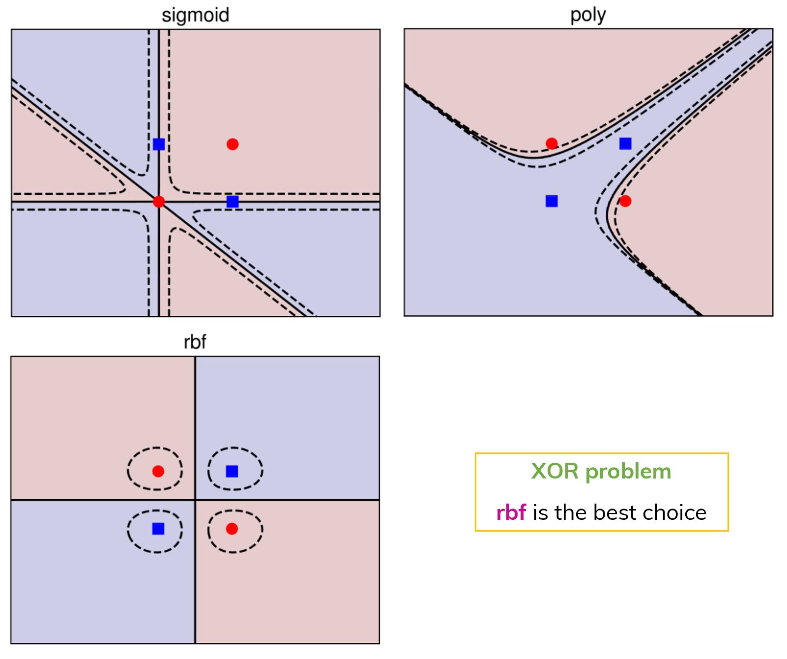
SVM in XOR problem. Using SVM with 3 different kernels in a XOR problem. In this case, Gaussian kernel is the choice.

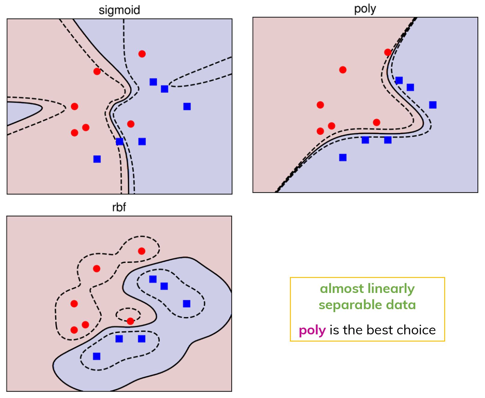
In the case of almost linearly separable data. Using SVM with 3 different kernels in the case of almost linearly separable data. In this case, Polynomial kernel is the choice.

Good or Bad?

Advantages:

  • Compared to both logistic regression and NN, a SVM sometimes gives a cleaner way of learning non-linear functions.
  • SVM is better than NN with 1 layer (Perceptron Learning Algorithm) thanks to the largest margin between 2 classes.
  • Accurate in high-dimensional spaces + memory effecient.
  • Good accuracy and perform faster prediction compared to Naïve Bayes algorithm.[ref]

Disadvantages:

  • Prone to overfitting: if number of features are larger than number of samples.
  • Don’t provide probability estimation.
  • Not efficient if your data is very big!
  • It works poorly with overlapping classes
  • Sensitive to the type of kernel used.

SVM used for?[ref]

  • Classification, regression and outliers detection.
  • Face detection.
  • Text and hypertext categorization.
  • Detecting spam.
  • Classification of images.
  • Bioinformatics.

Using SVM with Scikit-learn

from sklearn.svm import SVC

svc = SVC(kernel='linear') # default = 'rbf' (Gaussian kernel)
# other kernels: poly, sigmoid, precomputed or a callable

svc = svc.fit(X, y)
svc.predict(X)

# gives the support vectors
svc.support_vectors_ 

There are other parameters of sklearn.svm.SVM.

In the case of linear SVM, we can also use sklearn.svm.LinearSVC. It’s similar to sklearn.svm.SVG with kernel='linear' but implemented in terms of liblinear rather than libsvm, so it has more flexibility in the choice of penalties and loss functions and should scale better to large numbers of samples.[ref]

Meaning of some parameters

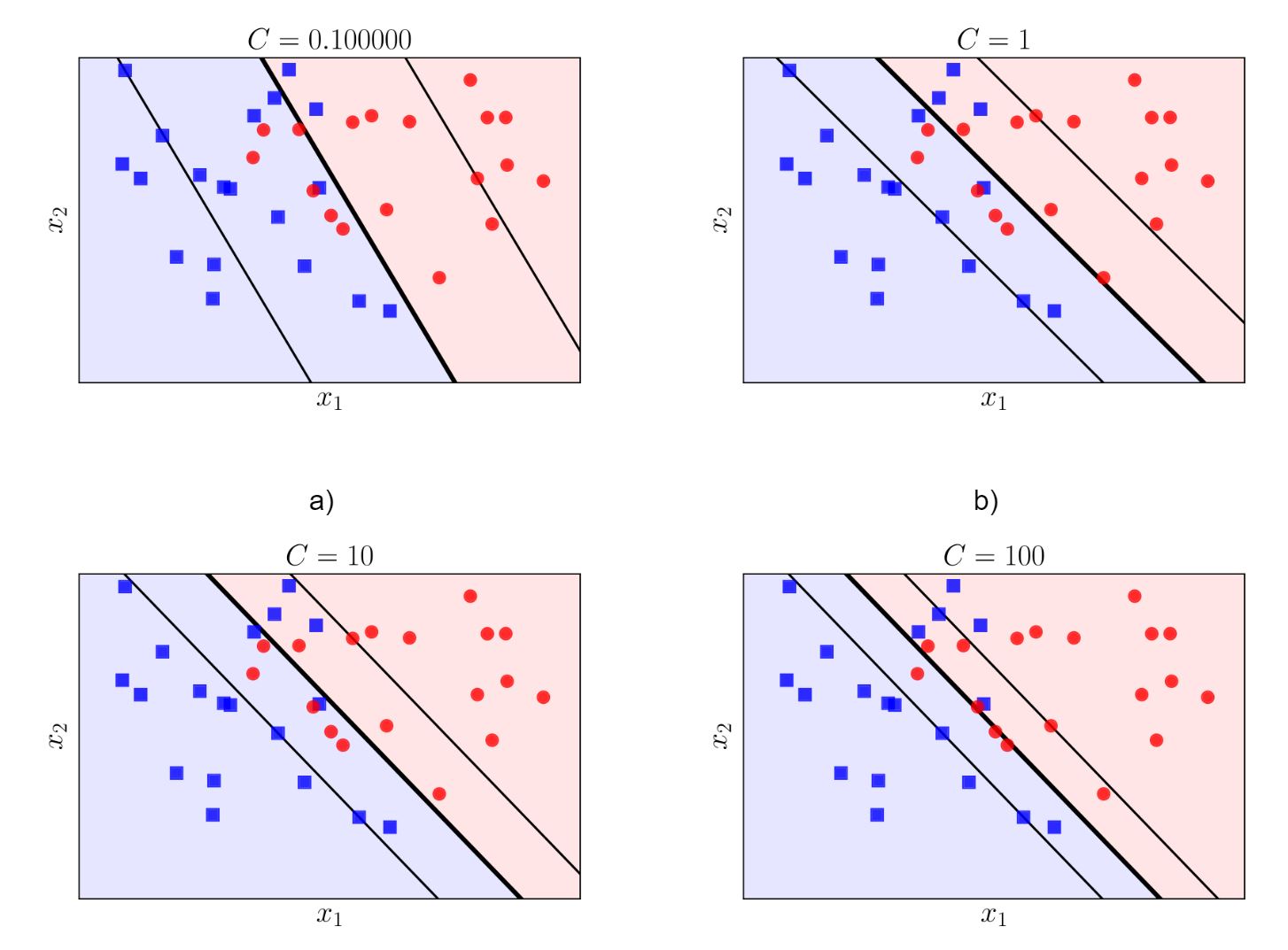
The Regularization parameter (C, default C=1.0): if C is larger, hyperplane has smaller margin but do a better job of classification and otherwise. This is how you can control the trade-off between decision boundary and misclassification term.

  • Higher values of C \Rightarrow a higher possibility of overfitting, the softmargin SVM is equivalent to the hard-margin SVM.
  • Lower values of C \Rightarrow a higher possibility of underfitting. We admit misclassifications in the training data

We use this in the case of not linearly separable data; It’s also called soft-margin linear SVM.
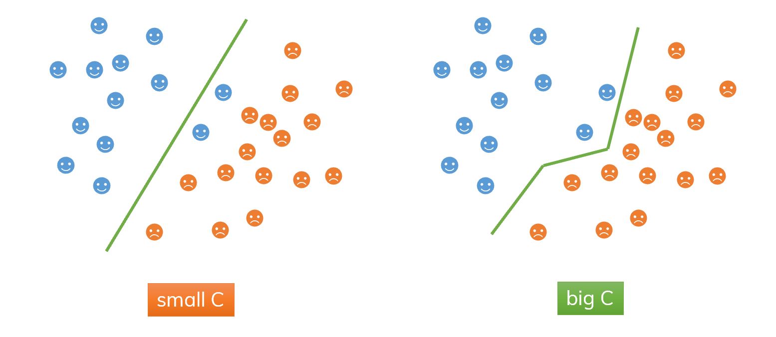
The Regularization parameter. An illustration of using C.

The Regularization parameter. An illustration of using C. Bigger C, smaller margin.[ref]

Recall that the hard-margin problem is,

(w,b)=argminw,b12w22subject to  yi(wTxi+b)10,i=1,2,,N.(4 revisited) \begin{aligned} &(\mathbf{w}, b) = \arg \min_{\mathbf{w}, b} \frac{1}{2}\Vert\mathbf{w}\Vert_2^2 \\ \text{subject to} &~~ y_i(\mathbf{w}^T\mathbf{x}_i + b) -1 \geq 0, \forall i = 1, 2, \dots, N. \end{aligned} \quad (4~\text{revisited})

and its duality is,

λ=argmaxλ(i=1Nλi12i=1Nj=1NλiλjyiyjxiTxj)subject to  λi0,i=1Nλiyi=0, i=1,,N.(5 revisited) \begin{aligned} &\lambda = \arg\max_{\lambda} \left( \sum_{i=1}^N \lambda_i -\frac{1}{2}\sum_{i=1}^N \sum_{j=1}^N \lambda_i\lambda_j y_i y_j \mathbf{x}_i^T\mathbf{x}_j \right) \\ \text{subject to} &~~ \lambda_i \ge 0, \sum_{i=1}^N\lambda_iy_i = 0, ~\forall i=1,\ldots,N. \end{aligned} \quad (5~\text{revisited})

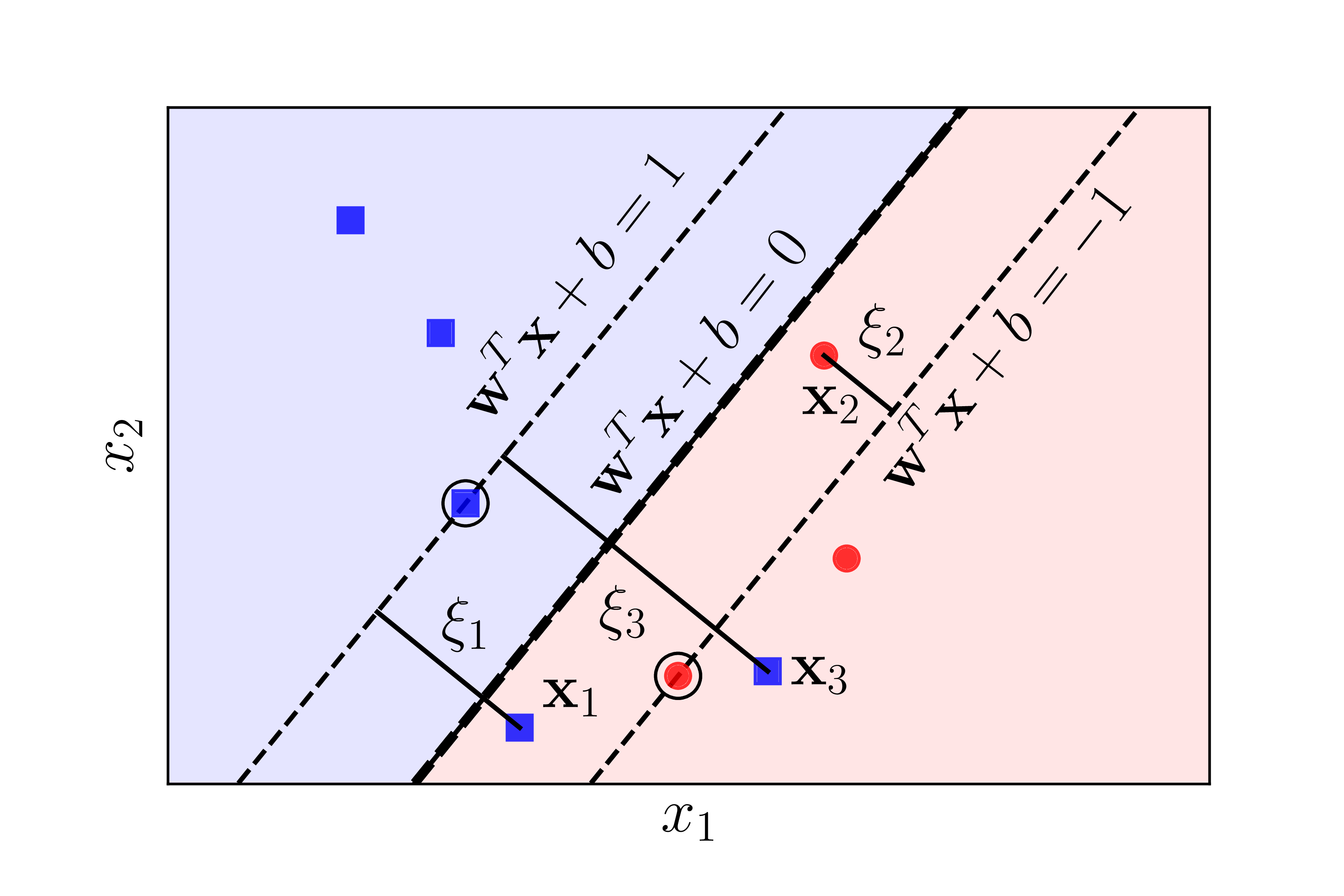
Instead of considering a hard-margin (4)(4), we consider following soft-margin problem (with the addition of slack variables)

The slack variables. An introduction to slack variables.[ref]

(w,b,ξ)=argminw,b,ξ(12w22+Ci=1Nξi)subject to  yi(wTxi+b)1ξi,i=1,,N  ξi0, i=1,2,,N \begin{aligned} &(\mathbf{w}, b, \xi) = \arg\min_{\mathbf{w}, b, \xi} \left( \frac{1}{2}{\Vert\mathbf{w}\Vert_2^2} + C \sum_{i=1}^N \xi_i \right) \\ \text{subject to} &~~ y_i(\mathbf{w}^T\mathbf{x}_i + b) \geq 1 - \xi_i, \forall i = 1, \dots, N \\ &~~ \xi_i \leq 0, ~\forall i = 1, 2, \dots, N \end{aligned}

With these new slack variables, we have to decide the trade-off between maximizing the margin (term 12w22\frac{1}{2}\Vert \mathbf{w}\Vert_2^2) and minimizing the mistakes (term CΣ1nξiC\Sigma_1^n\xi_i).

When CC is big, the term 12w22\frac{1}{2}\Vert \mathbf{w}\Vert_2^2 is almost considered as 00 in the minimized problem and the problem focuses on minimizing the term CΣ1nξiC\Sigma_1^n\xi_i (avoiding misclassification). That’s why the margin looks more narrow in the case of bigger CC.

A dual formulation of above soft-margin problem is,

λ=argmaxλ(i=1Nλi12i=1Nj=1NλiλjyiyjxiTxj)subject to  0λiC,i=1Nλiyi=0, i=1,,N.(6) \begin{aligned} &\lambda = \arg\max_{\lambda} \left( \sum_{i=1}^N \lambda_i -\frac{1}{2}\sum_{i=1}^N \sum_{j=1}^N \lambda_i\lambda_j y_i y_j \mathbf{x}_i^T\mathbf{x}_j \right) \\ \text{subject to} &~~ 0 \le \lambda_i \le C, \sum_{i=1}^N\lambda_iy_i = 0,~\forall i=1,\ldots,N. \end{aligned} \quad (6)

Note that, (6)(6) looks like (5)(5) (duality of hard-margin problem) but condition 0λiC0 \le \lambda_i \le C.

Gamma (gamma, default gamma='auto' which uses 1/n_features): determine the number of points to construct the hyperplane.
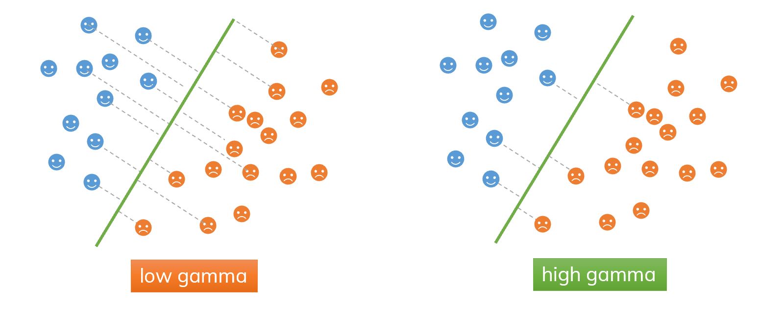
The parameter gamma. An illustration of using gamma. In low-gamma case, we only consider points nearby the hyperplane, it may cause an overfitting.
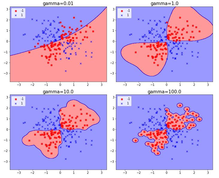
gamma parameter. Bigger gamma, more change to get overfitting (in a XOR problem).

We have another form of Gaussian kernel which is,

K(xi,xj)=exp(xixj22σ2), K(\mathbf{x}_i, \mathbf{x}_j) = \text{exp}\left( - \dfrac{\Vert \mathbf{x}_i - \mathbf{x}_j \Vert^2}{2\sigma^2} \right),

where σ\sigma is the standard deviation which shows the spread of the data.

Compare to the one used in the scikit-learn, K(xi,xj)=exp(γxixj2)K(\mathbf{x}_i, \mathbf{x}_j) = \exp(-\gamma\Vert \mathbf{x}_i - \mathbf{x}_j \Vert^2), we see that γ\gamma is an inverse of σ\sigma. It implies,

  • When σ\sigma is bigger (or γ\gamma is smaller), the similarity between two points xi\mathbf{x}_i and xj\mathbf{x}_j are considered in a wide range (spreading widely).
  • Conversely, when σ\sigma is smaller (or γ\gamma is bigger), only two points xi\mathbf{x}_i and xj\mathbf{x}_j which are really near to each other will be considered to be similar. That’s why we see there are many “groups” in the figure corresponding to γ=100\gamma=100. It leads to an overfitting problem.

SVM in action

  • XOR problem to see the effect of gamma and C in the case of using RBF kernel: Open this html fileOpen In Colab

  • Face Recognition[ref]: Open this html fileOpen In Colab

    • We will use a principal component analysis to extract 150 fundamental components to feed into our support vector machine classifier.
    • Grid search cross-validation to explore combinations of parameters.
    • For a real-world facial recognition task, in which the photos do not come precropped into nice grids, the only difference in the facial classification scheme is the feature selection: you would need to use a more sophisticated algorithm to find the faces, and extract features that are independent of the pixellation. For this kind of application, one good option is to make use of OpenCV, which, among other things, includes pre-trained implementations of state-of-the-art feature extraction tools for images in general and faces in particular.
    • I generally only turn to SVMs once other simpler, faster, and less tuning-intensive methods have been shown to be insufficient for my needs. Nevertheless, if you have the CPU cycles to commit to training and cross-validating an SVM on your data, the method can lead to excellent results.

References